Chapter 3. Phase 2: Extending the Model Showcasing the Power of Micro-simulation
In the second phase of model development, we extend typical population projections in the following ways for education, first union, fertility, provinces, and infant mortality:
- Education: Education is modeled and used for other processes as an explanatory variable. Currently the education module concentrates on primary education, central to current policy efforts in Mauritania, which does not provide universal access to primary education and has low retention rates. The model includes entry into primary and graduation from primary as key processes, extended by a distributional model of years of primary completed by school dropouts. The model works on the provincial level and can account for inter-generational transmission processes, i.e., children from higher-educated mothers having higher chances of entering and graduating from school. While useful for some policy applications in Mauritania, the model also provides a platform for refinement, e.g., by adding higher graduations.
- First union: The time of first union formation—which in Mauritania is marriage—is contained in many censuses in developing countries and is an important determent of fertility. It allows a better depiction of the concentration of reproduction: instead of distributing children to women independent of union status (especially in early life, e.g., 20 percent of females without schooling are married at or before age 14 in Mauritania), fertility is concentrated to fewer women, thus better reflecting reality. Change to union formation is one of the key mechanisms of fertility changes, as the age at first union increases fast especially for those entering higher education. This allows for addressing fertility change to various factors.
- Fertility: Fertility is modeled in detail and allows the user to choose a wide range of scenarios for alternative model implementations. The goal of detailed modeling is a realistic depiction of the distribution of family size. This requires modeling fertility by parity, time since last birth, as well as characteristics such as partnership status and education, a key determinant. In addition, the fertility module allows alternative alignment routines, reproducing given projections in aggregated outcomes, while adding realistic family sizes. Distribution of family size—the concentration of reproduction—may be of key policy relevance, as it is frequently those with the least education who have more children. Parity and education are also key explanatory variables for maternal and child mortality.
- Provinces: Mauritania has 13 provinces (i.e., Willayas) and most processes are modeled on the provincial level. The biggest Willaya is the capital, Nouakchott, with one-third of the national population; it also receives the most migrants—approximately 75 percent. Inter-provincial migration is modeled in alternative ways, with or without accounting for education, which considerably increases mobility in the Mauritanian case. As for other modules, the migration module can be a platform for model refinement.
- Infant mortabiilty: Infant mortality is modeled in some detail, using a list of explanatory variables including age and education of the mother. This allows for modeling downstream effects of educational investments and other potential policies to reduce infant mortality.
The following general design choices were made:
- We kept the model simple, transparent, and user friendly, selecting models that allow intuitive parameters. For example, we use probabilities, hazard rates, and odds ratios whenever possible, avoiding complex regression coefficients.
- We covered a variety of approaches typically used in micro-simulation, including hazard regression, logistic regression, life tables, and, in the case of first union formation, a parametric model which allows very intuitive parameterization, e.g., by setting average ages at union formation and the proportion of women expected to enter marriage over their lives, rather than measures that would require math to calculate such properties.
- We avoided conflicts between goals like simplicity, variety, and use of established models by implementing various alternative solutions in parallel when such conflicts arise, letting the user decide which approach to use. This will also help demonstrate and assess the impacts of alternative assumptions on the simulation results.
- We built and refined the model step-wise, and allowed switching some of the added processes on or off in the simulation, which offers a broad range of scenarios. For example, the model can be run with and without internal migration, and when adding education as a variable influencing migration risks, we can compare results, such as the size and education composition of sub-national populations, with simulations that do not account for education.
- Starting from an established macro model, we reproduced published projections. This can be done directly, as in step one, by using the same assumptions and reproducing the same processes, or indirectly, by aligning aggregated outcomes of the model to these targets, while adding detail and additional distributional information.
- We built the model as a platform that accepts future extensions, refinements, and modifications. The technical implementation is modular, allowing model builders to re-use code.
3.1. Primary Education
3.1.1. Discussion
In its current version, the education module focuses entirely on primary education. Three education levels are available: never entered primary school, entered primary school without completion, and completed primary school. In this way, modeling the decision on education outcome can be accomplished early in life, before other processes, such as union formation and first birth, for which education is used as an independent variable.
The model is driven by three probabilities: to graduate from primary education by year of birth, province of birth, and sex, which are entered respectively. As another dimension and model option, mother’s education can be added as a relative factor. When this option is chosen for a selected year of birth onward, the probabilities to enter and graduate primary education by mother’s education are “frozen” and all future changes are riven by the changing educational composition of mothers. This allows analysis of trends, as the relative differences by parents’ education are typically very persistent.
Modeling of primary education is only the start of modeling education; higher education may be the development priority of the model and primary education may serve as template. While the model is very simple, we implemented it in a way that allows extensions and refinements in many dimensions. For example, we implemented a separate primary school actor who selects students. This approach can be easily extended to model both the demand and supply side of schools and/or the demand for teachers on a regional level.
3.1.2. Parameters
The primary education module contains nine parameters:
- The probability to enter primary education by year of birth, sex, and province of birth
- The probability to graduate from primary education by year of birth, sex, and province of birth
- Primary school entry age
- Primary school graduation age
- Start of the school year
- Use of mothers’ education: on/off
- Log odds of entering primary education by mother’s education
- Log odds of graduating from primary education by mother’s education
- Year from which on mother’s education is introduced and for which the model is calibrated

Figure 3-1: Education Parameters
3.1.3. Analysis
The core models
The primary education module is based on four regression models. The first two—entering primary education and graduating from primary education—are based on census data and are used for the base scenario. In the second step, related models are estimated from MICS to estimate the influence of mother’s education, and mother’s education can then be added to the model as a proportional factor, allowing for a variety of scenarios. The key parameter tables for entering and graduating from primary school contain probabilities which were calculated from log odds estimated by logistic regression:
P = exp(estimated log odds) / ( 1 + exp(estimated log odds))
The base models are estimated from census data and use birth, sex, and year of birth as variables. Cohort trends are estimated using people between age 12 for primary school and 16 for secondary, and age 32. These trends are a good fit for the past and, due to the log transformation in logistic models, level off in the future, providing plausible base scenarios. Differences by province are very pronounced and persistent.
In the second step, odds ratios of primary and secondary school graduations by mother’s education are estimated from MICS. Users can run alternative scenarios in which overall trends in education progressions are replaced by the dynamics stemming from mother’s education. The application automatically calibrates results for a chosen base year of birth, so that the alternative scenario, including mother’s education, produces the same outcome as the trend scenario for the chosen year of birth.
As the model runs on a provincial level, education trends stemming from three sources can be distinguished:
- The changing composition of the population by province
- Changes in education stemming from the changing education composition of the mother’s generation
- Overall cohort trends
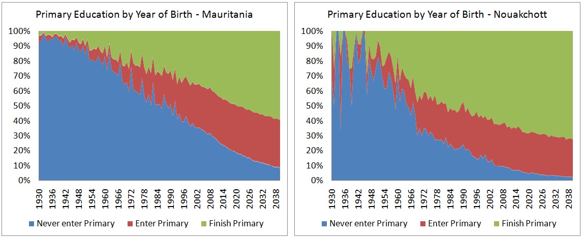
Figure 3-2: Highest School Attended, National and Nouakchott - Data and Projected Trends by Year of Birth
To detect gender-specific trends, separate logistic regressions by sex were estimated, including the population age 12-32 and dummies for province (at birth), assuming proportionality. Age 12 is used as the age cut-off, assuming that at this age everyone entering primary education has done so. Data show the lowest proportion of people without education at this age. There are considerable differences by province; the percentage of 12-year-olds who never entered formal schooling is between 15 percent in Nouakchott and 55 percent in Hodh Charghy. These two provinces also have the highest populations. Alternative scenarios could be created in which these gaps are closed. There are also gender differences; females have a steeper trend and recently overtook the males.
The model for primary school graduation follows the same logic, and the only difference is that age 16 was selected as the cut-off age, with the highest rate of people who have graduated from primary. Retention rates, which are the percentage of people staying in primary until graduation, are low, between 40 percent in Hodh Charghy and 70 percent in Nouakchott. Again, female trends are steeper, but male rates are still higher, especially in provinces with low retention rates.
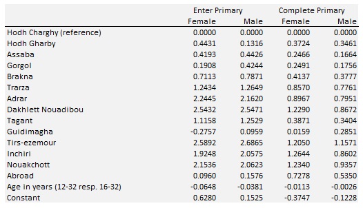
Table 3-1: Regression Results for Entry and Completion of Primary Education
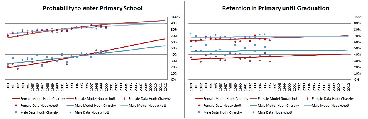
Figure 3-3: Primary Education by Year of Birth for Nouakchott and Hodh Charghy, Data and Projected Trends
Introducing Mother’s education
Models including mother’s education cannot be estimated from the census, so MICS was used to run the same models as above to control for differences by Willaya and extend by mother’s education. The estimated values are in line with literature; interestingly, mother’s education has a far higher impact for males.
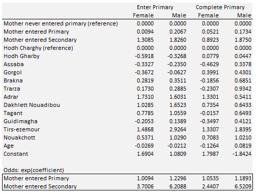
Table 3-2: Estimation Results for Odds by Mother’s Education (Data: MICS 2011)
Combining the census model with estimates for odds by mother’s education requires calibration to get the same probabilities for a given base year with and without introducing mother’s education. Technically, one searches for a calibration term (with the interpretation of an additional proportional log odds factor) by numeric simulation, which, for a given education composition of the mother’s generation, leads to the same graduation probability as the model without mother’s education. These calculations are done automatically within the model software.
Reproducing the model
- Stata code: 07_Education_MICS.do
- Excel parameter file and census analysis results: Education_Module.xlsx
- For analysis and regressions based on MICS data, run 07_Education_MICS.do. Result tables can be copied and pasted into the sheet MICS. This updates the graph of education by age and updates four regression models (enter and finish primary education by sex) used for calculating the parameters of odds by mother’s education.
- For analysis and regressions based on the census, run 06_Education_CENSUS.do and copy and paste result tables into the sheet CENSUS. Tables are education by age, regression results for entry, and success in primary education by sex (four models). There are eight other output tables used to produce graphical examples for two Willayas, Hodh Charghy and Nouakchott.
- All model parameters are calculated automatically in the sheet PARAMETERS, from which parameters can be copied and pasted directly into the application.
- The sheet SIMULATIONS can graphically compare the results of three alternative simulation results. Result tables from the application can be copied and pasted into this sheet to update all graphs.
3.2. Union Formation
3.2.1. Discussion
Changes in the age of first union formation is one of the key mechanisms behind fertility changes. Many developing societies currently experience a rapid increase in that age, partly resulting from educational expansion. In Mauritania and many developing countries, first union formation on average still occurs very early in life. Between 10 and 40 percent of females, depending on education, have entered a union by age 17; about 20 percent of women without any formal schooling enter a first union at or before age 14. Including this variable in the fertility model allows a better depiction of the concentration of reproduction: instead of distributing children to women independent of union status, fertility will be more concentrated to fewer women, especially at young ages, which better reflects reality.
From a modeling perspective, the fast-changing age profile in first union formation imposes interesting challenges. Fast demographic change, especially shifts in age profiles, make period data of limited use for modeling. For example, union formation rates decrease fast for the very young, but this observation does not necessarily mean that fewer people enter a union over the life-course, even if union formation rates are currently low at higher ages, where most of people observed today have entered a union already. It is in this environment when parametric models demonstrate their power. In our case, we implemented the Coale & McNeil approach for modeling entry into first unions. The parameterization of such a model is very intuitive; parameters are the minimum age at first union formation (currently around 10 in Mauritanian data), the average age, and the proportion of women who will eventually marry. We allow separate parameterization by primary education outcome. Period rates that result from fitting relevant models using these parameters are calculated within the application and displayed in output tables. Alternatively, to give users a broader choice in approaches, we allow period rates by education as model parameters. Also, the The Coale & McNeil model produces table output of union formation by age, which can provide feedback as a parameter for the second model. This can easily create scenarios of policies that set a minimum age at marriage.
3.2.2. Parameters
The module has three parameters:
- A model selection parameter choice between a Coale & McNeil model and a model based on age-specific hazard rates
- The parameter for the Coale & McNeil model: minimum and average age at first union formation, proportion of women ever entering a union by year of birth
- Union formation rates by year of birth and age
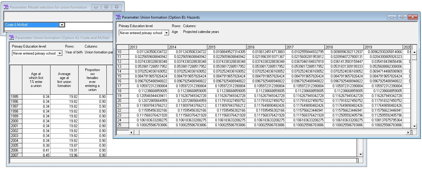
Figure 3-4: Union Formation Parameters
3.2.3. Analysis
Current period data
From a modeling perspective, the fast-changing age profile in first union formation imposes interesting challenges. Fast demographic change, especially shifts in age profiles, limit use of period data for modeling. When applying age-specific period data of first union formation as observed in the census, between 20 and 25 percent of women, depending on education, would never enter a union before age 40..
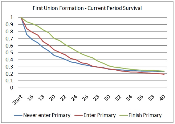
Figure 3-5: Current Period Survival
Hazard regression, including age-specific trends
Comparable results for period rates can be obtained by hazard regression, including age-specific trends. The following graph shows the very distinct age pattern in the most recent union formation hazards by education for observations between 2005 and the 2013 census.
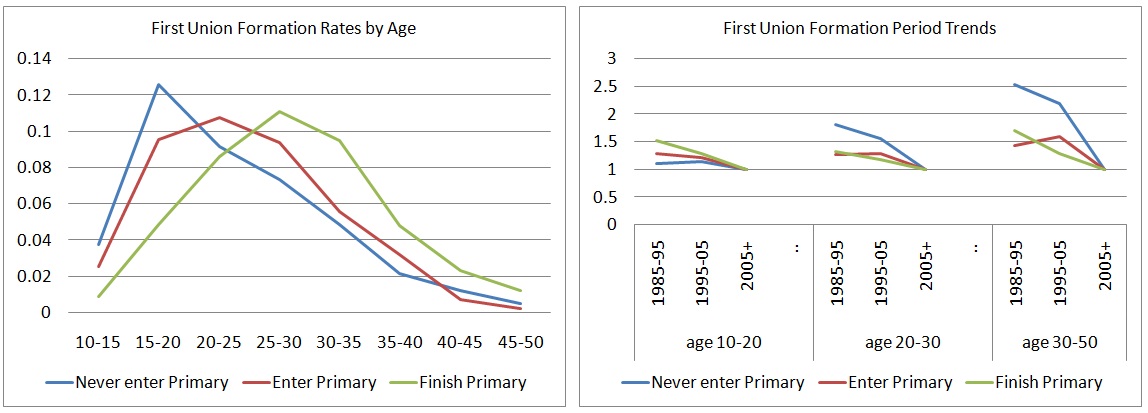
Figure 3-6: First union formation rates by age and time trends
Based on these rates, and creating a synthetic cohort living its entire life in the period 2005-13, almost 90 percent of women would eventually enter a first union. There are very steep trends. Relative period risks (reference 2005+) are decreasing for all distinguished age groups, but in reverse order by education and age group: rates below 20 were decreasing most significantly for more highly educated women, while for older age groups, rates decreased more for groups with less education.
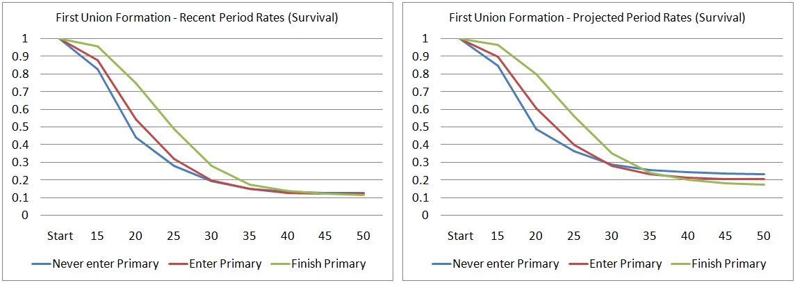
Figure 3-7: Recent Period Survival and Projected Survival 2015-2025
Past period trends are of limited use for informing future scenarios. It is expected that delays in union formation at lower ages will eventually lead to catch-up effects at higher ages, but this reversal in trends was not observed yet, using the broad age groups in this example. While “recent trend scenarios” are popular in micro-simulation, continuing the trend as observed in the past 10 years for another 10 years would double the proportion of women never entering a union.
Hazard regression by cohort
Displaying rates by birth cohorts makes the modeler’s choices visually more explicit: the younger the cohort, the shorter their observed behavior and the longer the remaining lifetime for which rates have to be modeled.
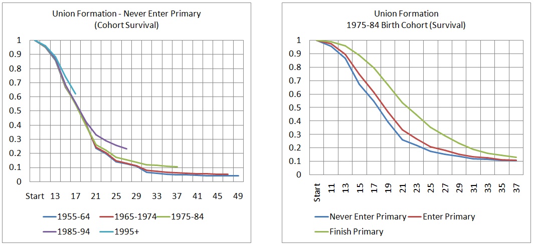
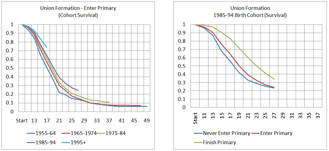
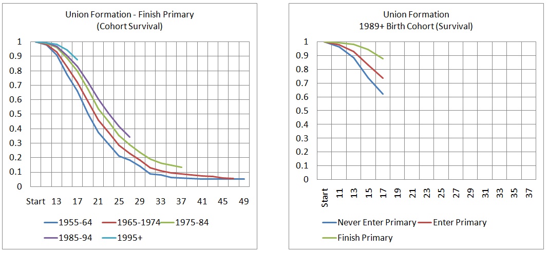
Figure 3-8: Cohort Survival
Parametric models
Besides “borrowing” from observed behaviors of older cohorts with or without applying trends, another approaches are parametric models to fit survival curves. Such a model was proposed by Coale and McNeil in the 1970s, based on extensive studies on the age pattern of first marriages in many countries. Their standard density of first marriage, constructed from pattern observed in Sweden 1856-9, has the form:
gs(x) = 0.19465*exp(-0.174(x-6.06) – exp(-0.288(x – 6.06)))
They found that a relational model with three parameters transforming the proportion of ever married at the age resulting from the above density function can fit most populations:
G(a) = C * GS ( ( a-a0 ) / k )
- a = age
- a0 = minimum age when the process starts (empirically, ~age where the first percent married)
- k = indicator of the spread of the distribution, i.e., how fast marriage occurs after a0 (how many years of the population’s schedule are equivalent to one year of the standard)
- C = the proportion of the population eventually entering marriage
Rodriguez and Trussell (1980) noted that k stands in direct relation to the average age at marriage µ, allowing parameterizing a model more intuitively with µ instead of k:
µ = ∫aG(a)da = a0+11.36k, thus k = (µ - a0)/11.36
Estimations for Mauritania: using the Excel Solver to fit the equations based on the survival curves provides remarkably good fits to data. Figure 3-9 shows fitted curves for women with secondary education as well as the cohort trends in average age at first union formation:
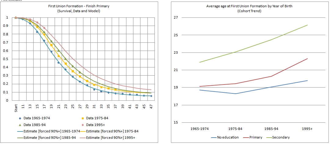
Figure 3-9: Solution for Coale and McNeil Model, Time Trends
The highest uncertainty (and room for scenario building) is probably in “guesses” for C. Almost equally good fits, especially for the youngest cohort, can be found fixing C at different levels.
In the context of the micro-simulation, this approach was implemented as a choice, side by side with a table of period rates, because it is probably more intuitive for scenario building. It allows for parameterization—by birth cohort, separately for each of the three education groups—by setting parameters for average age at union formation and the proportion of women ever entering a union. Scenarios for parameters for average age can be informed by recent trends or by international experience.
Reproducing the module
Stata Files:
- For analysis of current period probabilities, run 08_UnionFormation_Prob.do and copy the model results (three models by education) into the sheet PeriodProbabilities. This is for analysis only and not used in the application.
- For analysis of recent period rates and period trends, run 09_UnionFormation_Histories.do and copy the results, three hazard regression models by education, into the sheet PeriodHazard&Trends. This is for analysis only and not used in the application.
- For analysis of cohort survival, run the file 10_UnionFormation_Cohorts.do and copy and paste the estimation results, 15 hazard regression models by cohort and education, into the sheet Cohort Survival. These results are used for curve fitting to fit Coale and McNeil models. Curve fitting is performed using the Excel Solver to find solutions for three parameters: Start age, Average age at marriage, and Proportion eventually marrying. Solutions must be found for four cohorts for each of the three education groups. This is done in the three sheets (one by education): CohortNeverEnterPrimary, CohortEnterPrimary, CohortFinishPrimary. All three parameters can be searched for simultaneously, and parameters can be fixed, e.g., to force the model to produce a chosen target proportion of people ever marrying.
Excel
- All calculations and parameter are in the workbook: Union_Formation.xlsx
- The model Parameters are provided in the sheet PARAMETERS from where they can be copied and pasted into the application. This sheet also allows setting future target parameters (for 2050) and applies linear trends to reach them.
3.3. Alternative Models for Fertility
3.3.1. Discussion
While very popular, the use of period rates of age-specific fertility in population projections has three types of limitations:
- Even if it were possible to have perfect knowledge of future rates, the simulation would not produce realistic life-courses for women. Age as the only determinant of fertility would not lead to a realistic distribution of children to mothers and thus of family sizes. It ignores other determinants of fertility like parity, time of the last birth, union status, and education. So even with perfect foresight, we would obtain only the right number of babies. Micro-simulation can increase policy relevance of projections by placing newborns into their family context: their survival, future school attendance, etc., can take into account parents’ characteristics, which in return are relevant to the cost of policies.
- A projection tool based on age-specific rates cannot inform scenarios of fertility changes. Scenarios must be produced outside of the model, and often mechanically, by starting from observed rates, future target rates (e.g., from a country which underwent demographic changes earlier), and a transition path. Theories of behavioral changes are not made explicit nor are they distinguishable from composition changes. Micro-simulation allows the explicit modeling of behavioral changes, respectively, permits the study of composition effects in isolation. The latter can run status quo scenarios where changes in overall fertility arise entirely from changing composition of the population.
- Macro scenarios based on given rates do not allow modeling of feedback reactions and policy effects on fertility. For example, if highly educated women are expected to have fewer and later births, a micro-simulation model will naturally produce these downstream effects when running scenarios on educational expansion. Other scenarios could include legislation effects, e.g., the imposition of a minimum age of marriage.
To build and use the strengths of micro-simulation, we can derive the following modeling priorities:
- The capability to produce realistic life-courses for given overall rates. In this mode of model use, the focus is on the refinement of a macro model—a realistic distribution of children to mothers—without changing the macro assumptions on the future number of births.
- The capability to model and analyze scenarios of behavioral changes as well as composition effects.
- Scenario support for the modeling and identification/assessment of downstream effects of policies, like educational expansion or legislation of legal ages for marriage.
The refined fertility module was built around these priorities. First, we model births separately by birth order. In the case of first birth, age is kept as the main (baseline) factor, but age-specific birth rates are estimated separately by education group (expecting differences in the age pattern) and for women who ever entered a union and those did not (where fertility is very low).
For higher-order births, we estimate separate models for births of order 2-15. To model realistic birth intervals, the baseline is now the time since previous birth. Relative risks were added to capture the effects of education and broad age groups, for higher ages where fertility decreases considerably.
Users are given various model choices for model selection and alignment options. In particular, the refined model can be run with total births or total births by age aligned with the base model. This produces identical aggregate projections as found in published sources while respecting the relative differences in birth risks between women by parity, birth interval, education, and union status.
3.3.2. Parameters
The refined fertility module introduces four new parameters:
- Model selection: Users have four choices for modeling fertility
- Option 1: Using the base model; the refined module is disabled
- Option 2: Using the refined model without alignment
- Option 3: Using the refined model but aligning the aggregated number of births to the base models. While the relative fertility differences between women of different parity, education, union status and age are respected, the model is aligned (forced) to produce the same number of births as the base model. This produces the same aggregate scenarios, but adds detail leading to more realistic female life-courses.
- Option 4: Using the refined model, but aligning the aggregated number of births by age to the base models. While the relative fertility differences between women of different parity, education, and union status are respected, the model is aligned (forced) to produce the same number of births by age as the base model. This produces the same aggregate scenarios, but adds detail leading to more realistic female life-courses and is faster than Option 3, as at each birth event, only the most appropriate mother is searched within the age group.
- First birth rates by age, province, education, and union status
- Higher-order births: duration baseline and relative risks by mother’s age and education for births of order 2-15
- Period trends by parity
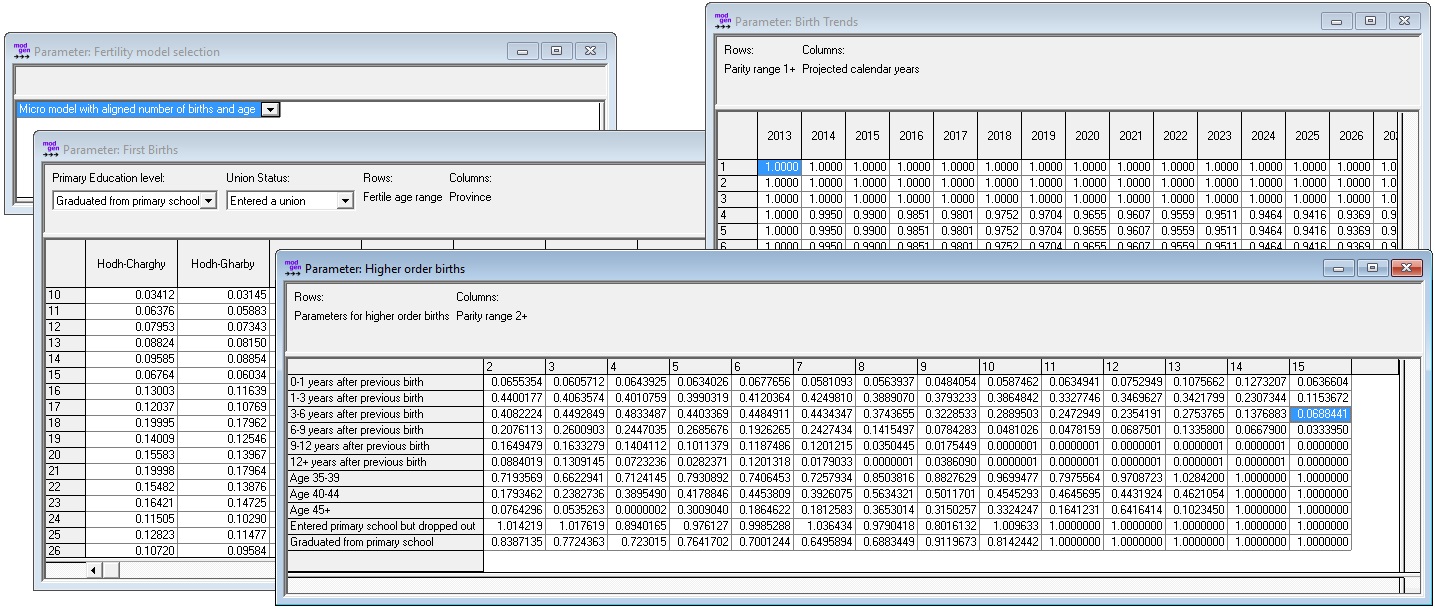
Figure 3-10: Fertility Parameters - Refined Version
3.3.3. Analysis
First births
First births are based on estimates from census data using the information on reported births in the past 12 months. Parameters are birth rates (hazards) by single year of age and province of residence, marital status (ever having entered a union), and the three education groups based on primary school entry and graduation. While the parameter consists of a single four-dimensional table, i.e., age, province, marital status, education, the respective rates are calculated from the log odds and estimated using logistic regression models:
- For women 15+ who ever entered a marriage, models by age and province are run separately for each education group, allowing for different age profiles by education.
- For women 15+ who never entered a marriage, due to a much smaller population and very low birth rates, education is added as proportional factor instead of estimating the model separately by education.
- Fertility below age 15 is estimated separately, as the influence of education and regional differences are different at this young age compared to women 15+.
- The models for first births of women below age 15 are estimated separately by marital status. Due to very small sample/population, inter-provincial differences are not estimated for women who never entered a marriage.
Higher-order births
For the second to the 14th birth, separate proportional hazard regression models are estimated from MICS data. This approach was chosen as the duration since last birth is a strong predictor of higher-order birth events and including this duration, which is not available from the census, allows more realistic modeling of birth intervals and thus female life-courses. Also, using event history data informs scenarios of future trends.
Reproducing the analysis
- Excel file of parameter tables and calculations: Refined_Fertility.xlsx
- Stata file for first births (based on census): 12_FirstBirthCensus.do
- Stata file for higher-order births (based on MICS): 13_HigherOrderBirthsMics.do
- Stata file: 11_MICS_CreateAnalysisFile.do creates the analysis file for higher-order births based on a file of women and a file of children. The file has the following variables:
File: m_mics_fertility.dta

Variables:

    - M_ID      Person ID (women)
    - M_BIRTH   Birth date (women)
    - M_WEIGHT  Record Weight
    - M_Bnn     Birth dates of children nn 01-14
    - M_EDUC    Primary education: never entered / dropout / finish level 5+
    - M_MAR     Date of first marriage
3.4. Infant Mortality
3.4.1. Discussion
Child mortality is a key policy concern in many developing countries. There is a wide body of literature on determinants, both individually, e.g., characteristics of the mother, and contextually, e.g., availability of health care infrastructure on the regional level. Micro-simulation can be a powerful tool for policy-relevant analysis and projections, as it can handle the detailed characteristics that drive child mortality. In this context, the presented model is just a starting point for detailed analysis. It takes two characteristics of mothers into account, mother’s age and education. In combination, we found child mortality 2.5 times higher for mothers who did not graduate from primary school and are under 15 years old.
The child mortality module is optional. If activated, it starts replacing the overall mortality model five calendar years after the starting year of the simulation, ensuring that all children “know” their mother’s characteristics (are born in the simulation). As mother’s characteristics are not available for children born outside the country, immigrants are excluded from the model and handled by the general mortality module.
3.4.2. Parameters
Four parameters were added to the base mortality module to model child mortality at a greater level of detail:
- A model selection parameter, with four model choices
- Disable the child mortality model: the same model as for all ages is used
- Child mortality model without alignment: the child mortality module replaces the overall mortality module for ages 0-4. Note that the overall life expectancy might be altered by this choice.
- Child mortality model calibrated for an initial year, then trends for other ages: in this choice, life expectancy is the same as in the overall mortality for the given year, but as the composition of the population by mothers’ characteristics changes over time, the number of deaths and therefore life expectancy will differ for the following years, allowing for scenario comparisons.
- Child mortality model calibrated for an initial year, then specific trends from the child mortality module: Here, life expectancy is the same as in the overall mortality for the given year, but as the composition of the population by mothers’ characteristics changes over time, and as a result of potentially different trends, the number of deaths, and therefore life expectancy, will differ for the following years, allowing for scenario comparisons.
- Baseline risks for child mortality (reference category mothers above 16 and graduated from primary school)
- Relative risks for child mortality by child’s age, mother’s age (group) at birth and mother’s education
- Time trend for child mortality by age
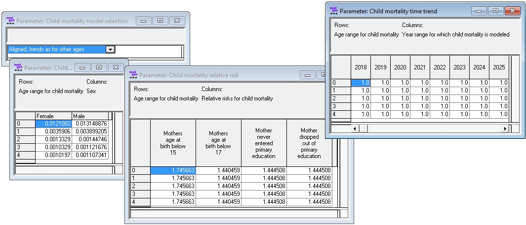
Figure 3-11: Child Mortality Parameters
3.4.3. Analysis
Data analysis is based on the file m_mics_childmortality.dta generated from MICS and containing the following variables:
m_mics_childmortality.dta

    - M_BIRTH       Date of birth (months since 1900)
    - M_DEATH       Date of death (months since 1900)
    - M_MALE        Sex (Male = 1 / Female = 0)
    - M_WEIGHT      Weight
    - M_AGEMO       Age of mother at birth (in months)
    - M_EDUCMO      Primary education of mother (0 never entered, 1 dropout, 2 graduate)
    - M_INTERV      Date of interview (months since 1900)
- Stata file: 16_MICS_AnalysisChildMortality.do
- Parameter calculation and tables Excel file: ChildMortality_Module.xlsx
Baseline hazard and relative risks were estimated simultaneously by a proportional hazard regression model. There were not any significant difference between not having entered primary school at all and having dropped out from primary school, so we collapsed the two groups.
/*
    ANALYSIS OF CHILD MORTALITY
    DATA FROM MICS MAURITANIA
    MARTIN SPIELAUER, 2016
    Input file: m_mics_childmortality.dta
*/

/*
-------------------------------
 Wrapper function stpiece
 -------------------------------
 the following adds the wrapper function stpiece which can be used to make code more efficient;
 without this function, time splits of the baseline duration have to be done manually;
 it was developed by Jesper B. Sorensen Nov. 20 1999;
 the function can be added to Stata, download at: http://fmwww.bc.edu/repec/bocode/s/stpiece.ado;
*/

    clear all
program define stpiece
    version 6.0
    syntax [varlist(default=none numeric)] [if] [in] ,  ///
                   [tp(numlist >=0) tv(varlist) PREsplit(integer -1) noPREserve *]
    if "`preserv'"=="" {
        preserve
    }
    if "`presplit'" == "-1" {
        if "`tp'"=="" {
            display in red "You must either declare data to be presplit or use tp()"
            exit 198
        }``
        display in gr "Invoking stsplit..."
        quietly stsplit tp, at(`tp')
        display in gr "Creating time pieces..."
        quietly tab tp, gen(tp)
        local i = _result(2)
        drop tp
    }
    else {
        local i = "`presplit'"
    }
    if "`tv'" ~= "" {
        display in gr "Creating interaction effects..."
        tokenize `tv'
        while "`1'" ~= "" {
            local stub = substr("`1'",1,4)
            local j=0
            while "`j'" < "`i'" {
                local j = `j'+1
                local x = "tp`stub'`j'"
                quietly generate  `x'=`1'*tp`j'
            }
         mac shift
        }
    }
    streg tp* `varlist' `if' `in' , nocons d(e) `options'
end

    /*******************************************/
/* Settings and file of birth records      */
/*******************************************/
clear
#delimit;
use "m_mics_childmortality.dta";

/*******************************************/
/* Variables                               */
/*******************************************/

    generate RecNo = _n;
/* Person died - this is the event studied */
generate ChildDied = 0;
replace  ChildDied = 1 if M_DEATH != .;
/* Observation time */
generate DUR = ( M_INTERV - M_BIRTH ) / 12.0;
replace  DUR = ( M_DEATH - M_BIRTH ) / 12.0 if ChildDied == 1;
/* Censor at age 5 and drop cases with death after age 5 */
replace ChildDied = 0 if DUR > 5;
replace DUR=5 if DUR>5;
/* Mothers age group at birth */
gen AgeGrMo = 2;
replace AgeGrMo = 1 if ( M_AGEMO / 12.0) < 17.0;
replace AgeGrMo = 0 if ( M_AGEMO / 12.0) < 15.0;
char AgeGrMo[omit]2;
/* Mother graduated from primary school */
gen MothNoPrim = 0; replace MothNoPrim = 1 if M_EDUCMO < 2;

    /*******************************************/
/* Episode splitting                       */
/*******************************************/

stset DUR, failure(ChildDied) id(RecNo);
/* splitting file in period episodes */
stsplit After1980, after at ( 0 10 20 30) ( time = 1980 - (1900 + M_BIRTH /12.0) );
replace After1980=4 if After1980==30;
replace After1980=3 if After1980==20;
replace After1980=2 if After1980==10;
replace After1980=1 if After1980==0;
replace After1980=0 if After1980==-1;
label define After1980
  0 "Before 1980"
  1 "1980-1989"
  2 "1990-1999"
  3 "2000-2009"
  4 "2010+";
label values After1980 After1980 ;
char After1980[omit]4;

    /*******************************************/
/* Estimation                              */
/*******************************************/
xi: stpiece i.After1980 i.AgeGrMo i.MothNoPrim i.M_MALE, tp( 1, 2, 3, 4 );
3.5. Migration refinements
3.5.1. Discussion
Analysis shows higher rates of migration for more highly educated people, with different magnitudes of effects by province. The option to simulate migration by education is added in this modeling phase. Micro-simulation can be a powerful tool for the detailed simulation of migration decisions on the individual and family levels. Such models can include contextual information on regions (e.g., public infrastructure, such as the availability of schools) as well as regional events like droughts and climate change. From that perspective, the presented models can be starting points for more detailed, policy-relevant modeling.
3.5.2. Parameters
Two parameters were added to the base module:
- A selection parameter allows a choice between the base module and the refined module modeling migration by education
- A table of migration probabilities by education, sex, age group, and province
Tables used from the base module are:
- The on/off switch, to model migration
- A table of migration probabilities by sex, age group, and province (applied if the base module is selected by the user)
- The distribution of destination provinces by sex, age group, and province of origin
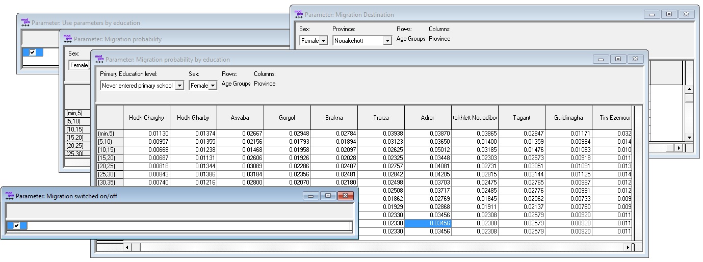
Figure 3-12: Internal Migration Parameters Including Internal Migration by Education
3.5.3. Analysis
We applied logistic regression models estimated separately by education group and sex. The impact of education is very different by province; for example, in the capital, Nouakchott, migration rates are very low and independent of education. For other provinces, migration rates are up to five times higher for primary school graduates compared to people who never entered primary education. When mechanically applied in the simulation, this effect will both accelerate the growth of Nouakchott and influence the educational composition of it population.
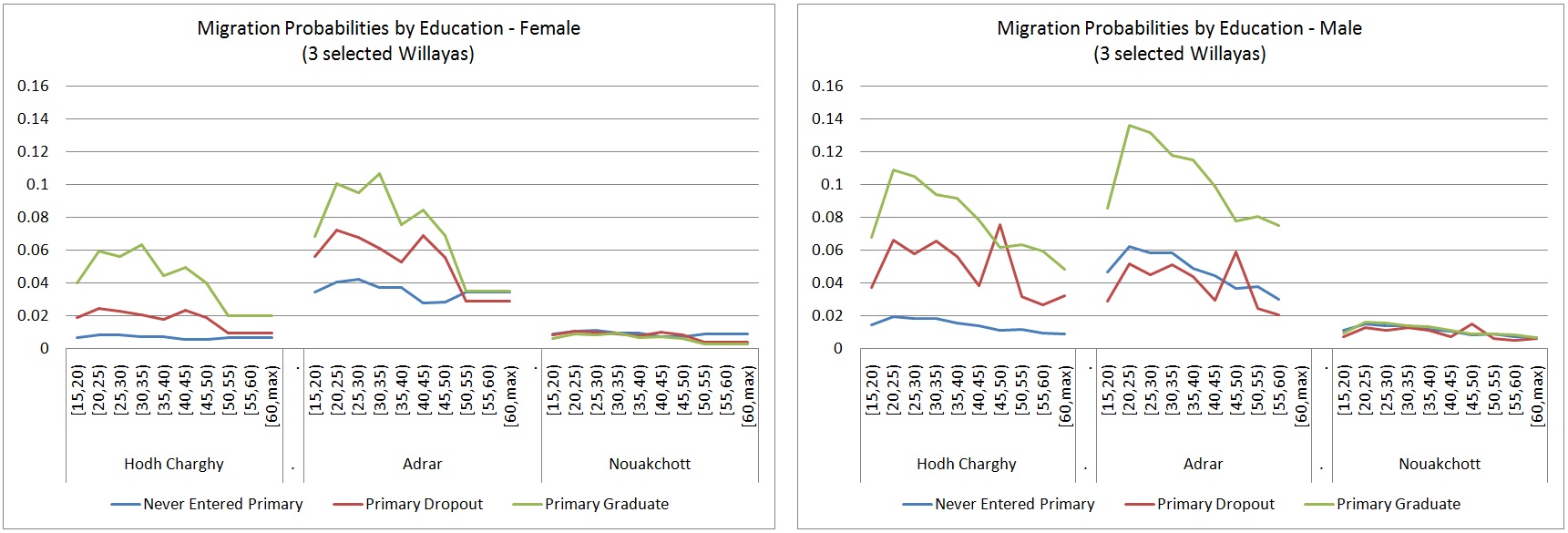
Figure 3-13: Internal Migration
3.5.4. Reproducing the Analysis
- Stata code: 17_MigrationRefined.do
- Excel parameter file: Refined_Migration.xlsx