Chapter 2. Phase 1: Reproducing a Typical Macro Population Projection Model
In this and the following section, we develop and describe a two-phase micro-simulation model for population projections. In the first phase, we implement a typical cohort-component macro-projection model, DemProj, as a micro-simulation model. In the second phase, we exceed the capabilities of macro models by adding additional processes, variables, and features and demonstrate some of the key strengths of micro-simulation. The purpose of this exercise is fourfold:
- To provide a projection model for Mauritania with policy relevance in key priority development areas such as child mortality, education, and the management of migration flows
- To provide a portable model, which can be customized for other countries and adapted or refined for additional applications
- To demonstrate the usability and versatility of such a model from a user’s perspective
- To provide a step-by-step manual covering key modeling aspects, parameter estimation, and application programming
Components of a population projection are a representation of the current population—e.g., a micro-data file or a distributional table—and a model for moving this population forward. Key elements replicated from DemProj at this step are models for fertility, internal migration, international migration, and mortality. This model will be further developed in the next section by adding modules for education, first union formation, and child mortality, and by refining the modules for fertility and migration.
2.1. The Base model: Reproducing a macro model
We chose to start the development of a population projection micro-simulation model by reproducing the typical macro model DemProj. While such an exercise does not immediately add anything to DemProj, there are benefits to this approach:
- We demonstrate that a micro-simulation implementation of a population projection model based on the cohort-component method is a relatively straightforward process and an alternative way to implement the same model.
- We help lower the entry barrier to run micro-simulation models from a user’s perspective by providing a familiar model with parameter tables and results identical to the DemProj macro model. The model can be used as a training tool to introduce features of the user interface common to all Modgen models.
- By producing projections that are identical to published macro projections, the model produces benchmarks that can also be useful in the following model refinements and steps, both for comparison of results and as alignment targets. In the latter case, micro-simulation is used to add detail to projections (e.g., a realistic distribution of family sizes by education) while reproducing aggregate outcomes (e.g., number of births) as projected by cohort-component models.
- From a technical perspective, the micro-simulation implementation of DemProj introduces most key concepts of micro-simulation programming and the modules can be used as typical building blocks of micro-simulation models.
- In addition to all the demonstrative reasons listed above, the micro-simulation implementation of DemProj also provides a good and logical starting point for model extensions beyond the capabilities of macro models. It already implements the core modules of a population projection model based on the population representation by individual actors, which can be easily refined by adding individual-level characteristics, additional events, and communication and interactions between actors.
The data needed in this phase are identical to those of a macro population projection model. In the case of Mauritania, scenarios for fertility and mortality were supplied by the National Statistical Office (ONS). Data sets for individual countries, including Mauritania, and regions can also be downloaded from DemProj project sites (e.g., http://www.healthpolicyproject.com/index.cfm?id=software&get=Spectrum). The ONS currently does not include international migration in its macro projections, and provincial distributions are input into national projections. In contrast, we explicitly include internal migration, emigration, and immigration in the micro-simulation. (All corresponding models can be disabled by users.) Current measures for internal migration, immigration, and emigration were calculated from a sample of census data. The estimation of approximate emigration was based on census records of household members who recently left the country.
2.2. Starting Population
2.2.1. Discussion
DemProj, as a cohort-component model, is cell based. Cells are defined by all possible combinations of individual characteristics, such as age, sex, and province, and the model’s population information is represented by the count of people in each cell, i.e., a table of persons by age, sex, and province. Technically, the same approach can be used to start a micro-simulation model; there are two possible ways: directly, producing one person or a multiple of clones for each person on the table, or using the table to sample the characteristics of simulated actors. The latter approach is more common and more flexible, as it allows the user to choose the sample size. It is also typically sufficient to run a sample of a population and allows scaling of the model.
This approach has the same limitations as all cell-based models: by adding characteristics, the number of cells explodes exponentially. For example, a model by single age 0-100, sex, 13 provinces of residence, 14 provinces of birth (including abroad), 6 education groups, a range of children (parity) 0 - 15, and 4 categories of marital status would have 101 x 2 x 13 x 14 x 6 x 16 x 4 = 14.12 million cells—in our case, a number four times the population of Mauritania. Cell-based models would have to identify all possible transitions between each cell and model transition probabilities, an unfeasible task that limits the number of characteristics that can be handled by this approach to very few.
From a micro-simulation perspective, representing a population by multidimensional distributional tables is useful only if the storage space of such a table does not exceed a micro-data file containing the same information. In addition, a cell-based representation of a population does not allow continuous variables, e.g., income, and would have to split them into categories. Using a micro-data file to start a simulation is thus the most common approach in micro-simulation, which is typically used for detailed modeling. The exception to this rule—complex models starting from distributional tables—are so-called synthetic models, such as the Canadian LifePaths. In this case, all persons are created with very few characteristics sampled from distributional tables, and other characteristics are modeled from birth over the life-course, starting the simulation in the past. Seen as an imputation technique, modeling characteristics longitudinally can be used as a micro-simulation application by itself (reconstructing the past) and models for the past can be kept to project characteristics into the future (if it adequately reproduces the past). A second way for adding missing characteristics consists of cross-sectional imputations at the beginning of the simulation. Cross-sectional imputations are usually performed outside of the micro-simulation model by tools like SimPop, which was used to prepare the starting population file of our application in its second development step. Here, in a first step, the starting population is represented by a three-dimensional table of the population by age, sex, and province, with information from the 2013 census.
Another design choice in micro-simulation is when to start the simulation of each actor. This can happen in the past, thus creating all actors with age 0 and aging them until the starting point of the simulation, or creating actors at the starting moment of the simulation, with the age and all characteristics at this moment in time. The first approach allows the type of longitudinal imputations of characteristics described above and is thus more flexible in giving people individual histories. In our case, given the simplicity of the model, both approaches work. To demonstrate the implementation of both approaches, we create all persons of the starting population at age 0, but create future immigrants “on demand” at the moment of immigration. While the former approach in Step 2 will also be used to impute some past information, such as school graduations, the latter is used to demonstrate cross-sectional imputations of missing information, e.g., by sampling missing variables from the resident population or recent immigrants with otherwise identical characteristics.
2.2.2. Parameters
The starting population of the base version of the model is contained in a single parameter table by age, sex, and province.
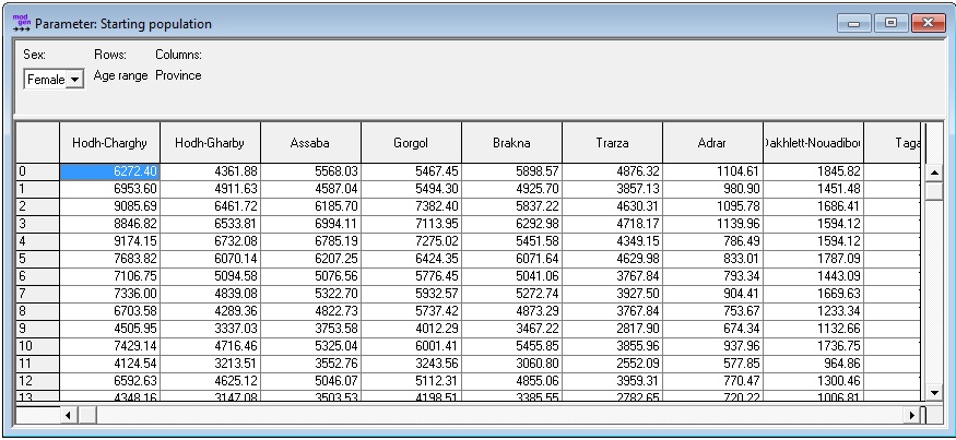
Figure 2-1: Starting Population Parameter
2.2.3.Analysis
The starting population parameter is tabulated from the population census file.
- Stata file: 02_StartingPopulations.do
- Excel Parameter Tables: Starting_Population.xlsx
/* ************************ */
/* DATA RESIDENT POPULATION */
/* ************************ */

clear all
#delimit;
use "Microdata\m_census_residents.dta";

/* ************************ */
/* DISTRIBUTIONAL TABLE     */
/* ************************ */

gen M_NAGE = int(M_AGE);

tab M_NAGE M_POR [iweight=M_WEIGHT] if M_MALE == 0;
tab M_NAGE M_POR [iweight=M_WEIGHT] if M_MALE == 1;
2.3. Fertility
2.3.1. Discussion
The fertility module is based on age-specific fertility rates calculated from two parameters: an age distribution of fertility and the TFR for future years. In this parameterization, the model directly follows the DemProj approach, which splits fertility projections into one of age patterns and another of TFRs. The third parameter is the sex ratio.
The quality of the projections relies on the quality of the chosen fertility rates, and a wide body of literature exists for how to project fertility patterns. Typical patterns and trajectories were identified and are typically applied for developing countries, e.g., assuming common development stages of fertility transitions. The macro approach itself is limited to model fertility by age. Age is an important predictor for fertility itself, but also important for modeling maternal and child mortality, as those risks are far higher at both age extremes of the fertile cycle.
The implementation of this approach is straightforward in micro-simulation, where the same parameters of age-specific fertility are used in the macro projection to determine the number of births added to the population each year and are applied to individual women. Births are modeled in continuous time, thus can happen at any moment of time. For each woman age 15-49, a random waiting time to the next birth is calculated from the age and period-specific fertility rates calculated from the parameters. As rates are updated at each birthday and calendar years change, a birth event occurs and a new actor is added to the simulation if the waiting time is shorter than the time to the next update of rates, otherwise a new waiting time based on the new rate is generated, and so forth. At the birth event, the sex of the baby is determined by sampling from the sex ratio parameter. The province of birth as well as the moment of birth are information transmitted from mother to child.
Modeling fertility exclusively by age does not result in a realistic representation of female birth histories and the distribution of family sizes as it ignores important other individual characteristics, like marital status, the current family size, education, and the time since last birth. Some of these characteristics will be modeled and added in the second step of model development, adding both realism and policy relevance to the model.
2.3.2. Parameters
The fertility module is based on age-specific fertility rates calculated from two parameters: an age distribution of fertility and the TFR for future years. In this parameterization, the model directly follows the DemProj approach, which divides fertility projections into projections of age patterns and of total fertility rates. The third parameter is the sex ratio.
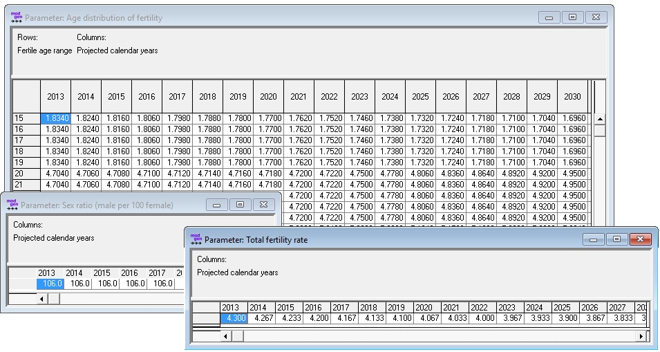
Figure 2-2: Fertility Parameters. (1) Age Distribution, (2) Sex Ratio, (3) Projected TFR
Unlike DemProj, which works with fertility distributions by five-year age groups, the micro-simulation implementation allows parameters by single years of age. While this allows for future refinements and provides more flexibility, the current parameterization reproduces DemProj.
2.3.3. Analysis
All parameters were provided by the Mauritanian ONS for the years 2013 through 2043. From there on, age patterns and sex ratio are kept constant, while total fertility rates are pro-rated, continuing a linear trend until reaching a rate of 2.0, which is kept stable. Data sets for individual countries, including Mauritania, and regions can also be downloaded from DemProj project sites (e.g., http://www.healthpolicyproject.com/index.cfm?id=software&get=Spectrum).
Current fertility rates can be estimated from census data if a link between 0-year-old children and their mothers can be established or women report births in the past 12 months. The first approach, the own child approach - assumes that babies stay with their mothers, who can be identified in the household. The approach can be refined by correcting for biases due to mortality. The second approach models fertility from the mother’s side. An example of estimating fertility rates from census data can be found in Chapter 3.4.
- Excel Parameter Tables: Base_Fertility.xlsx
2.4. Mortality
2.4.1. Discussion
Mortality is modeled and implemented following the approach in DemProj, i.e., by working with a standard mortality table for age patterns and a projected period of life expectancy. Within the application, the life table is scaled automatically for each year to meet the targeted life expectancy by calendar year and sex. Like fertility, mortality is modeled in continuous time, thus death can occur at any moment.
Life tables are central tools in demography, and extensive literature exists in mortality projections. As a consequence, although projections are available from various sources based on various methods, they are typically based on persistent patterns of mortality reduction observed in many countries over the past century. As for other processes, micro-simulation can add detail to mortality projections, e.g., by accounting for the observed and typically very significant and pronounced influence of education, marital status, or, in detailed models, health status and individual diseases. Micro-simulation is especially powerful for modeling inheritable and transmittable diseases e.g., HIV, as it can model interactions between actors.
Note that due to the separate parameterization of the age profile of mortality and life expectancy, changes in age profile alone do not result in changes in overall life expectancy, as the life table is automatically scaled to produce a targeted life expectancy. For example, lowering child mortality in the age profile would increase mortality at other ages to compensate for the effect. In the second step of model development, we allow for scenarios that improve on child mortality without re-scaling mortality at other ages, to “open” the model for the detailed modeling of child mortality by characteristics like mother’s education or parity.
2.4.2. Parameters
The two parameters of the base version of the model are a standard life table and projected life expectancy.
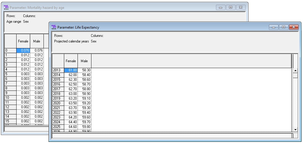
Figure 2-3: Mortality Parameters
2.4.3. Analysis
Data for this model were provided by ONS. Data sets for individual countries, including Mauritania, and regions can be downloaded from DemProj project sites (e.g., http://www.healthpolicyproject.com/index.cfm?id=software&get=Spectrum). In general, two sets of model life tables are employed by DemProj: the CoaleDemeny (Coale, Demeny, and Vaughan, 1983) model and the United Nations tables for developing countries (United Nations, 1982). Projections of life expectancy can have various sources: national projections, national goals, UN and U.S. census bureau projections, recent trends and international experience projections, or an application of the UN model schedule of mortality improvements.
Excel Parameter Tables: Base_Mortality.xlsx
2.5. Internal Migration
2.5.1. Discussion
As typical in macro models, migration is modeled using origin-destination matrices by age group and sex. For easier parameterization and scenario building, migration transitions are modeled here in two steps. The first is the probability to leave a province by current province of residence, five-year age group, and sex. The second step is the decision where to move, based on origin-destination matrices for movers by departure province, age group, and sex. While internal migration can be switched off in the model, it otherwise assumes the same migration rates in the future—a typical assumption in population projection models.
Analyses show higher rates of migration for more highly educated people, with different magnitudes by province. In the second modeling phase, the option to simulate migration by education is added. Micro-simulation can be a powerful tool for detailed simulation of migration decisions, both on the individual and family levels. Such models can include contextual information on regions (e.g., public infrastructure, like the availability of schools) as well as regional events like droughts and climate change. From that perspective, the models can be starting points for more detailed, policy-relevant modeling.
2.5.2. Parameters
The base migration module has three parameters: an on/off switch to disable migration; modeling, probability tables to migrate by age group, sex, and province; and the distribution of destination provinces by province of origin, age group, and sex.
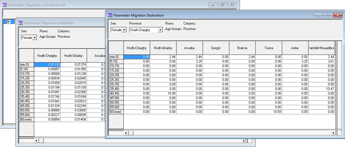
Figure 2-4: Internal Migration Parameters
2.5.3. Analysis: Estimating the Parameters
The ONS of Mauritania currently uses a Demproj version without internal migration; no “ready-made” official migration transition data are currently available. This gap is closed by estimating the model based on a census sample. Due to sample size restrictions, logistic regression is used to estimate probabilities to leave. This assumes a common age profile of migration risks for all provinces, which differ by the same proportional factor over all ages. Depending on age, between 60 and 80 percent of migrants move to the capital Nouakchott, which itself has only low rates of out-migration. Migration probabilities are very different between provinces; for some provinces and age groups (20-35), they reach or even exceed 10 percent.
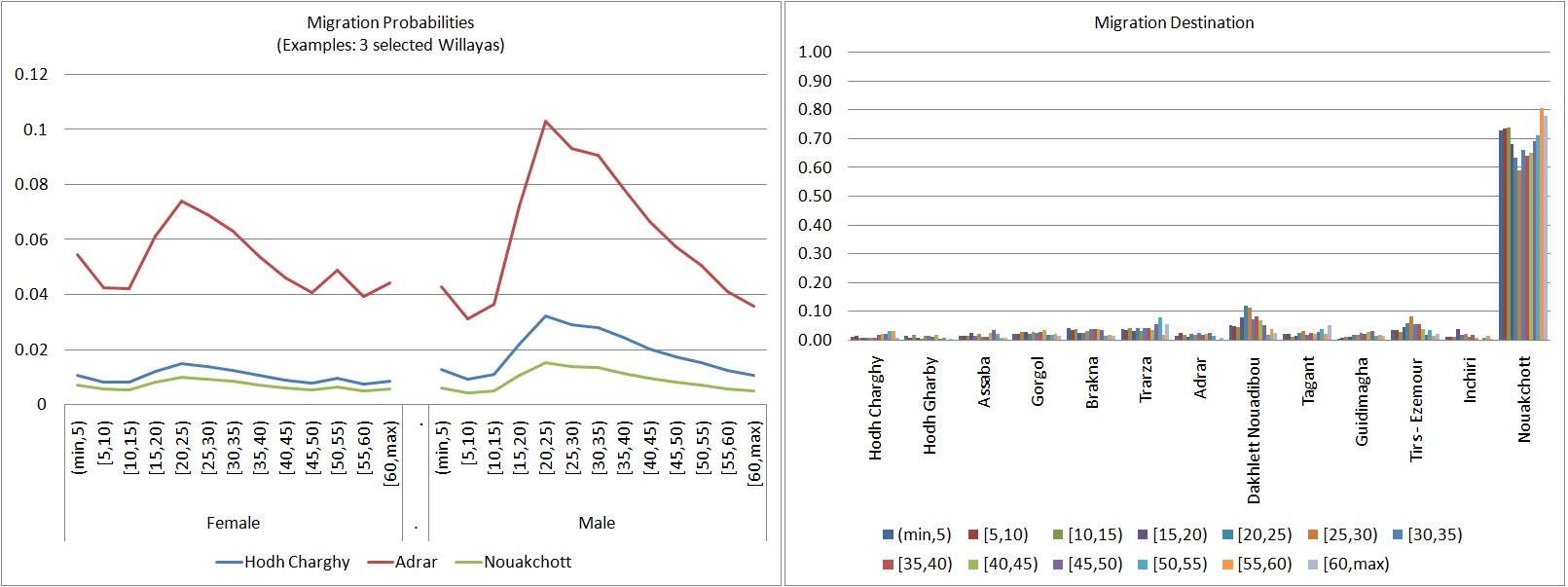
Figure 2-5: Migration Probabilities (3 Provinces) and Destinations
- Stata code file: 03_BaseMigration.do
- Auxillary data: m_empty_migrants.dta
- Excel parameter file: Base_Migration.xlsx
The model of probabilities to leave that currently uses logistic regression can be replaced by cross-tabs when running the analysis on the full census. The transition matrices are cross-tabs. To fill all cells of the transition matrix, a file with very low-weighted movers was created, allotting one person by sex and age group for each possible residential move. The code to append this file can be removed when running the analysis from the full census.
The essential code:
/* ************************* */
/* DATA: RESIDENT POPULATION */
/* ************************* */

clear all
#delimit;
use "Microdata/m_census_residents.dta";

/* ************************* */
/* VARIABLES                 */
/* ************************* */

/* Age one year ago, drop if < 0 */
gen m_ageago = int(M_AGE)-1; drop if m_ageago < 0;

/* Age groups 5 years ago, up to 60+ */
gen m_agegr5 = 5 * int(m_ageago / 5); replace m_agegr5 = 60 if m_agegr5 > 60;

/* Person is internal migrant (moved within the country)*/
gen is_migrant = 0; replace is_migrant = 1 if M_PPROV != M_POR & M_PPROV != 13;

/* Append (very) low weighted transition records of all possible transitions to avoid empty cells */
append using "m_empty_migrants.dta";

/* Person is potential migrant (not a recent immigrant) -- drop others */
drop if M_PPROV == 13;


/* ************************* */
/* MODELS                    */
/* ************************* */

/* Leaving */

xi: logit is_migrant i.m_agegr5 i.M_PPROV [iweight=M_WEIGHT] if M_MALE == 0;
xi: logit is_migrant i.m_agegr5 i.M_PPROV [iweight=M_WEIGHT] if M_MALE == 1;

/* Destinations by origin */

by M_PPROV M_MALE, sort : tabulate m_agegr5 M_POR [iweight = M_WEIGHT] if is_migrant, nolab row nofr;
2.6. Immigration
2.6.1. Discussion
As is typical for macro models, immigration is modeled by total projected numbers by year, age, and sex distribution of immigrants, and the distribution of destination provinces by age and sex. In the current implementation, only the parameter for total numbers of immigrants has a calendar time dimension. The age and destination distributions are assumed to be time invariant.
Similar to macro population projection models, the base version of the model does not provide immigrants with characteristics other than age and sex, but can be easily added as entities in the simulation. Modeling of immigration can become a complex and interesting issue in more detailed micro-simulation models. In our case—in the second phase—additional characteristics will be education, parity, date of first union formation, and time of last birth. There are alternative ways to create these characteristics, including simulation of immigrants from birth or the cross-sectional imputation of missing characteristics at the moment of immigration. We have chosen a very simple cross-sectional imputation method, consisting of sampling characteristics from the foreign-born host population. Such an approach will be sufficient if numbers of immigrants are relatively low and their characteristics do not differ much over time. The simulation of immigration can become a central focus in population micro-simulation in more detailed models, including immigration policies (selecting immigrants e.g., by education) or refugee migration.
2.6.2. Parameters
The model has four parameters: an on/off switch to allow simulations with and without immigration; total number of immigrants by sex and calendar year; age distribution of immigrants by single year of age and sex; and distribution of destination provinces of immigrants by sex and five-year age groups.
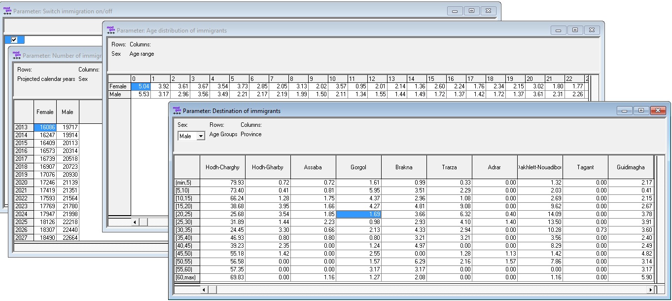
Figure 2-6: Immigration Parameters
2.6.3. Analysis
The ONS of Mauritania currently uses DemProj without immigration and no “ready-made” official immigration data are currently available. This gap is closed by using a 12 percent sample of the 2013 census to model immigration. The immigration module is based on census observations of immigrants having entered the country in the 12 months prior to the 2013 census. Based on estimates from the sample, the total number of immigrants is 37,000. This number contains a high number of refugees from Mali: 72.56 percent female and 63.00 percent male. Of those, 92.15 percent female and 80.20 percent male arrive in Hodh Charghy. According to local experts, it is supposed these immigrants will stay, but no new immigrants from Mali are expected. To account for that, we assumed a 95 percent drop in this immigration group. Such a scenario results in a total number of immigrants of 12,800. There is an interesting difference in the destination of immigrants by age: Nouakchott over-proportionally receives people in the active age range, while very young and older people are over-represented in Hodh Charhy.
Immigrants are defined as those who have lived in the current Willaya less than a year and previously lived abroad. Babies age 0 are treated as immigrants if they were born abroad. For those currently above age 0, a 50 percent probability is assumed, that their full age in years was one year younger at immigration. The model uses simple census cross-tabulations. In the simulation, all immigrants arrive at mid-year.
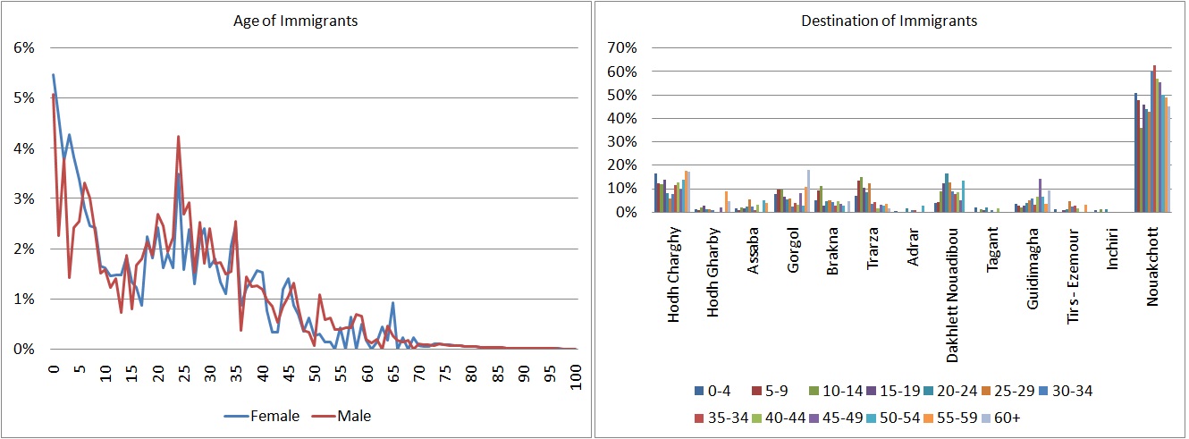
Figure 2-7: Age Distribution and Destination of Immigrants
- Stata code: 05_Immigration.do
- Excel parameter file: Immigration_Module.xlsx
- Auxilliary file: m_empty_immigrants.dta
To fill all cells of the destination matrices, a file with very low-weighted movers was created, allotting one person by sex and age group for each possible destination. The code to append this file can be removed when running the analysis from the full census.
/* ******************************** */
/* DATA: IMMIGRANT POPULATION       */
/* ******************************** */

clear all
#delimit;
use "D:\Dropbox\WorldBank2016_MS\Census\m_census_immigrants.dta";

/* ******************************** */
/* VARIABLES                        */
/* ******************************** */

/* Age at immigration: 50% chance of having been a year younger
   The high number of 0 year old is unrealistic, 50% are given a random age < 10
*/
gen m_age = int(M_AGE);
replace m_age = m_age-1 if runiform()<0.5; replace m_age = 0 if m_age < 0;
replace m_age = m_age + int( 10 * runiform() ) if m_age== 0 & runiform()<0.5;
tab m_age;

/* 5 year age groups, age at immigration, up to 60+ */
gen m_agegr5 = 5 * int(m_age / 5);
    replace m_agegr5 = 60 if m_agegr5 > 60;
    label define l_agegr5
        0 "0-4"
        5 "5-9"
        10 "10-14"
        15 "15-19"
        20 "20-24"
        25 "25-29"
        30 "30-34"
        35 "35-34"
        40 "40-44"
        45 "45-49"
        50 "50-54"
        55 "55-59"
        60 "60+" ;
    label values m_agegr5 l_agegr5;

/* Append (very) low weighted records of all possible destinations to avoid empty cells */
append using "D:\Dropbox\WorldBank2016_MS\Census\m_empty_immigrants.dta";

/* ******************************** */
/* VARIABLES                        */
/* ******************************** */

/* TAB 01: Number of immigrants by sex */
tabulate M_MALE [iweight = M_WEIGHT];

/* TAB 02: Destination of immigrants */
by M_MALE , sort : tabulate m_agegr5 M_POR  [iweight = M_WEIGHT], row nofr;

/* TAB 03: Age distribution of immigrants by sex */
tabulate m_age M_MALE [iweight = M_WEIGHT], col nofr;
2.7. Emigration
2.7.1. Discussion
Emigration is modeled by age-specific emigration rates by province and sex. Because emigration is not a priority of this report, this simple module will be kept in the second phase of model development. Similar to migration and immigration, micro-simulation can be a powerful tool for a detailed modeling of emigration. This may be relevant to developing countries in which emigration is frequent and relatives living abroad may aid resident relatives and contribute to development by remittances. On the negative side, brain drain might constitute a considerable problem for some societies and can be modeled specifically using micro-simulation.
2.7.2. Parameters
In addition to an on/off-switch, the only parameter for emigration is a table of emigration rates by province, age group, and sex.
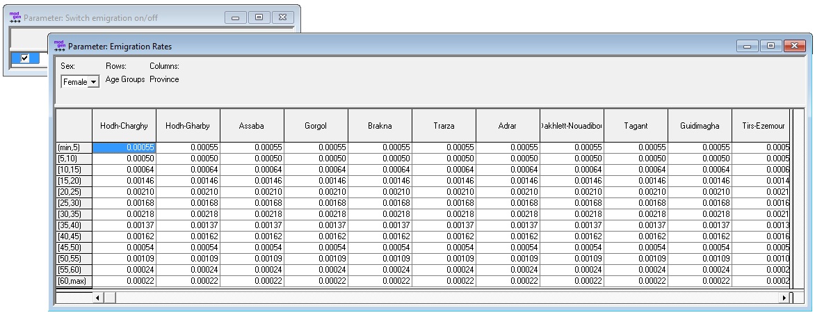
Figure 2-8: Emigration Parameters
2.7.3. Analysis
- Stata code: 04_Emigration.do
- Excel parameter file: Emigration_Module.xlsx
For immigration, the ONS of Mauritania currently uses DemProj without emigration and no “ready-made” official emigration data are currently available. This gap is closed by using a 12 percent sample of the 2013 census to model emigration.
Emigration rates by five-year age groups were calculated from 2012 departures from households reported in the 2013 census. Following this approach, only emigrants who leave part of the household are covered. Due to sample size restrictions and other data quality issues, we currently parameterize the model on the national level only. In the available sample, 88 percent of emigrants are male. Calculating survival of staying in the country from these period observations and ignoring back migration assumes that 50 percent of males would have left the country at age 60. Similar to internal migration and immigration, the model allows the option to switch emigration off.
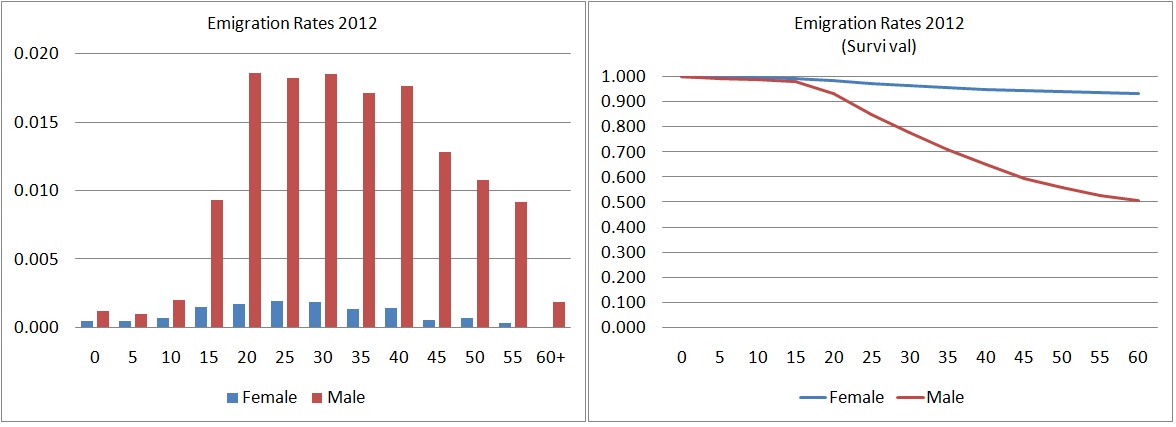
Figure 2-9: 2012 Emigration Rates
The parameters are based on two simple tables calculated from the census file version, including recent emigrants.
/* ******************************** */
/* DATA: POPULATION INCL. EMIGRANTS */
/* ******************************** */

clear all
#delimit;
use "Microdata\m_census_all_incl_emigrants.dta";

/* ******************************** */
/* VARIABLES                        */
/* ******************************** */

/* Age 12 months ago, drop if not born then */
gen m_age2012 = int(M_AGE)-1; drop if m_age2012 < 0;

/* 5 year age groups */
gen m_agegr = int(m_age2012 / 5) * 5;

/* identify emigrants */
gen m_emigrate = 0; replace m_emigrate = 1 if M_POR==13;

/* ******************************** */
/* ANALYSIS                         */
/* ******************************** */

tab m_agegr m_emigrate [iweight = M_WEIGHT] if M_MALE==0;
tab m_agegr m_emigrate [iweight = M_WEIGHT] if M_MALE==1;