Chapter 1. Rationale, Methods, Implementation, and a Portable Application
1.1. Introduction: Purpose, Scope, Organization
Population projections are key for policy making and planning. Changes in the size and composition of the population are key determinants of the demand for goods and services, from basic food and education, to energy and housing. Population projections, based on multiple scenarios, help government and other decision makers make informed decisions.
Most countries and international organizations, like the World Bank and the United Nations, produce population projections using the cohort-component method, a macro approach limited to a very small number of characteristics. This provides projections by age and sex at the national level, often dis-aggregated by urban/rural areas; large countries sometimes provide projections at a sub-national level. Given the high importance of education on human capital and its influence as the “single most important variable besides age and sex” on demographic behaviors (Lutz et.al. 1999), population projections that included education later became available for most countries, but that extension defined the technical limit of this approach.
A more advanced—but still uncommon—approach consists of dynamic micro-simulation models, in which populations are represented by large samples of individual people and their life-courses over time. This approach is more complex, but it has major advantages: it can produce detailed projections of a broad variety of individual characteristics, model realistic life-courses and their diversity, and support the modeling of interactions between people. The idea is to start with a micro-data population and make it evolve over time, unlike the cohort-component approach, which starts with a simple distribution of a population by age and sex but cannot track individuals over time. The idea is not new (van Imhoff and Post, 1998), but it has become feasible only recently, because advances in freely available programming technologies and improvements in available data have reduced costs. Micro-simulation models also allow more disaggregation and thus can provide projections of the population or some of its componentss, e.g., population by ethnic affiliation, school-age population by region, labor force by education level, etc. In addition, population micro-simulation models can provide the demographic core and foundation for more specialized micro-simulation models of diseases, tax benefit models, pension models, etc. A micro-simulation population projection model is used by Statistics Canada to project the diversity of the Canadian population by visible minority group (Caron-Malenfant et.al. 2010), Aboriginal identity (Morency et.al. 2015), and labor force (Martel et.al. 2011), as well as to study the effect of educational improvements on the future size and composition of the Aboriginal labor force (Spielauer 2014).
Population micro-simulation can be seen both as a complement to macro-projections and as their replacement, as macro-projection models can be implemented as micro-simulations, producing identical results, but allowing for model extensions beyond the technical limitations of cohort-component models. This point is demonstrated in this report with a micro-simulation example developed in two phases. The first phase reproduces the macro model DemProj (Stover & Kirmeyer 2001), which is widely used, especially in developing countries. In our example, we use Mauritanian data for its parameterization. In the second phase, the model is extended to incorporate more detailed characteristics and behaviors. Again we based the model on Mauritanian data sources, for which equivalent data are available throughout the world. Extensions include the fertility module, which allows a realistic projection of family sizes and fertility by education. We also added a module for child mortality, incorporating factors such as the mother’s education and number of siblings. Education is modeled to include its inter-generational transmission; first union formation is introduced as key determinant of the timing of first births.
This report is an attempt to demystify micro-simulation and, to a lesser extent, synthetic population, and demonstrate its feasibility in developing countries. The Mauritania example is key to this report, and includes detailed instructions for its adaptation and replication in other countries. The model is implemented in Modgen, a freely available software package developed and maintained at Statistics Canada. This package is compatible with a recent open source implementation of the same programming language under the name openM++. For the baseline population, we used a synthetic (or “virtual”) population generated using simPop (an open source R package). This approach allowed us to combine information from various data sources (in our case, the 2013 Population and Housing Census and the Multiple Indicators Cluster Survey 2011) into one data file and make these micro-data non-confidential.
The model also introduces micro-simulation programming and various statistical methods used in micro-simulation, and includes step-by step documentation of its computer implementation. The model has an intuitive graphical user interface and runs on a standard PC. Its code and statistical analysis files are openly accessible and can be used for micro-simulation model development and implementation. New software solutions, which are free, and improved computer capabilities make it an affordable and much more feasible option for developing countries. Given the growing interest in disaggregated data for development planning and monitoring (for example to monitor the Sustainable Development Goals), it makes sense to also push for more disaggregation in projections and simulations. Besides producing more detailed projections, micro-simulation also allows a more explicit incorporation of theory and policy levers in its projections. For example, it allows modeling of inter-generational dynamics and analysis of downstream effects on demographic change or child mortality of policy interventions that improve education.
This report has four parts:
- Background and Overview: The first part, Chapter 1. Rationale, Methods, Implementation and a Portable Application, introduces dynamic micro-simulation and its rationale for population projections, defines data requirements, and introduces the portable application and its user interface.
- Application Example: The second part details the portable model example, and Chapter 2. Reproducing a Typical Macro Population Projection Model and Chapter 3. Extending the Model Showcasing the Power of Microsimulation describe the population projection model applied to Mauritania. The first phase reproduces a typical macro model. In a second phase, we add modules, variables, and processes beyond the macro framework to illustrate key features and strengths of the micro-simulation approach. Parameter tables and the required data analysis for each module that replicates the calculation of model parameters are discussed. Links to all Stata files and a set of Excel files are also provided. The result is both a fully functional model that can be customized for other countries, as well as an illustration of typical modeling approaches found in micro-simulation. The model can also be understood as a modeling platform, allowing for extensions. Some modules contain parallel implementations of the user’s modeling options, which allows for a wide range of scenarios and assumptions. Scenario building and use of the model for projection analysis is demonstrated in Chapter 4. Using the model.
- Technology: This part discusses technological aspects of building micro-simulation models. Chapter 5. Microsimulation Technology: Modgen/OpenM++ discusses the technical implementation of the model from both a user’s and a developer’s perspective, thereby introducing the key components of the Modgen/OpenM++ programming technology and resulting applications. Chapter 6. Statistical Models Common in Microsimulation discusses the statistical models and concepts used in the example and introduces key methods widely used in micro-simulation.
- Materials: This part provides all materials to reproduce the sample model. Chapter 7. A Step-by-Step Guide for Implementing DYNAMIS-POP-MRT is a detailed documentation of the model code that model builders can use for micro-simulation model development and implementation. Each step discusses the model functionality, explains new programming concepts, and discusses the programming code. Finally, Chapter 8. Software Downloads describes and provides all necessary software downloads, including the micro-simulation model, programming resources, and statistical analysis files.
Data requirements are met by many countries—through their population censuses, and implementation of demographic household surveys like UNICEF’s Multiple Indicators Cluster Surveys (MICS) and Demographic and Health Surveys (DHS)—and we expect improvements on specialized modules. Once built and compiled, using the model is easy, as it has an intuitive graphical user interface and runs on a standard PC. While model development remains a complex issue, a collection of modular components that can be adapted and assembled for various purposes is being built. While it will not be a plug-and-play tool and still require technical expertise for model development or customization, this collection of well-documented modules should save developers and data analysts considerable time and lower the entry barrier into micro-simulation modeling.
References
Caron-Malenfant, E.; Lebel, A. & Martel, L. (2010), *Projections of the Diversity of the Canadian Population 2006 to 2031*, Statistics Canada Catalogue no. 91-551-X. [PDF]
Lutz, W., J.W. Vaupel, and D.A. Ahlburg, Eds. (1999) *Frontiers of Population Forecasting*. A Supplement to Vol. 24, 1998, Population and Development Review. New York: The Population Council.
Martel, L., É. Caron Malenfant, J.-D. Morency, A. Lebel, A. Bélanger, N. Bastien (2011) *Projected trends to 2031 for the Canadian labour force*, Statistics Canada Catalogue no. 11-010-X, vol. 24, no. 8 [HTML]
Morency, J-D, É. Caron-Malenfant, S. Coulombe, S. Langlois (2015) *Projections of the Aboriginal Population and Households in Canada, 2011 to 2036* - Statistics Canada Catalogue no. 91-552-X [PDF]
Spielauer, M. (2014), *The relation between education and labour force participation of Aboriginal peoples: A simulation analysis using the Demosim population projection model*, Canadian Studies in Population 41(1-2), 144–164.[PDF]
Stover, J., S. Kirmeyer (2001), *DemProj Version 4 - A Computer Program for Making Population Projections*, The POLICY Project Spectrum [PDF]
Van Imhoff, E. & W. Post (1998), *Microsimulation methods for population projection*, Population 10(1), 97–136. [PDF]
1.2. The Dynamic Micro-simulation Approach
Micro-simulation in the context of socioeconomic applications can be perceived as an experiment with a virtual society of thousands—or millions—of individuals. Micro-simulation models can be static or dynamic. Central to dynamic micro-simulation is the explicit modeling of the time dimension, following people and their families or households over time, rather than performing a before-and-after comparison in response to changes in the tax-benefit system or economic shocks. Dynamic modeling lends itself naturally to the modeling of policies with a longitudinal component, e.g., educational investments, especially in the context of general rapid social, economic, and demographic change that make it difficult to assess the contribution of individual policies to overall trends without tracking and comparing the lives of individuals who form a society.
This report advocates for dynamic micro-simulation, which has become increasingly feasible due to technical advances. Dynamic micro-simulation complements traditional evaluations of effects of development programs, given the context of the many development issues that evolve and impact individuals, families, and households over time and generations.
1.2.1. Advantages
Micro-simulation is attractive both from a theoretical and a practical point of view, as it supports research embedded into modern paradigms, such as the life-course perspective, while simultaneously providing a tool for what-if analysis of high policy relevance. Typical application areas include tax-benefit analysis, analysis of pension system adequacy and sustainability, and health and health insurance. One recent development is using micro-simulation in demographic projections. Although this has been discussed in literature for almost two decades (e.g., Imhoff & Post 1998), larger-scale implementations are a recent development. Statistics Canada was the first statistical office to produce official population projections using micro-simulation. Called Demosim, this model is implemented using the micro-simulation programming technology Modgen, which Statistics Canada developed. Modgen is freely available and shared worldwide. Variants of Demosim are currently being developed for several European countries as well as Australia (Belanger, forthcoming).
In social sciences and economics, there is an increasing emphasis on processes rather than static structures. This is where dynamic micro-simulation is most effective, as it can simultaneously deal with distributional and dynamic issues, e.g., demographic change, and with a longitudinal dimension to distributional analysis. From a policy perspective, there is increasing emphasis on processes rather than static structures; it also reflects the modern way of assessing poverty as a multi-dimensional and dynamic phenomena to be addressed by policies that go beyond static redistribution of resources, enable people to leave this state, and reduce poverty risks permanently. Micro-simulation can improve understanding of the complex dynamics resulting from many simultaneous processes, which are often studied only in isolation. In this context, dynamic micro-simulation is a key component in the evolution from analysis to synthesis (Willekens 2001) and can integrate analyses of single processes into computer simulations of societies. Such models can then be used for what-if analysis and assess how the future is shaped by today‘s decisions, policies, and actions.
In principle, whenever a system is made up of small-scale units, micro-simulation is an optional simulation approach. Micro-simulation has the potential to be especially powerful in three scenarios (Spielauer 2011): population heterogeneity, aggregation of behavioral relations, and individual histories.
Population heterogeneity
Micro-simulation is the preferred modeling choice when population heterogeneity matters and there are too many possible combinations of characteristics to split the population into a manageable number of groups.
Using a large sample of members to represent a population is an intuitive way to capture the population’s diversity and allows for distributional analysis of the effects of changes and reforms. Creating such a representation in a database of individuals is a typical step in micro-simulation development. Frequently, it will combine and integrate data from various sources, which ultimately makes data more relevant for policy analysis. It also allows policies to be targeted to very specific segments of the population.
From a longitudinal perspective, micro-simulation can capture the variety and heterogeneity in life-course experiences and careers, adding a whole new dimension in distributional analysis with the use of lifetime measures and capture of distributional impacts of policies over the individual life-cycle and between cohorts and generations. Besides its typical use for distributional analysis, micro-simulation can also track different ethnicities or minorities, which often display persistent behavioral differences over time, such as demographic behaviors. Individual modeling can improve the accuracy of projections. Besides persistence in differences, another frequently observed or theorized phenomenon (e.g., in modernization theory) is that behavioral changes are adapted by different groups at different times, and that certain sectors of society lead this development and are followed by others. The ability to model such processes can improve the theoretical foundation of projections.
The problem of aggregation
Micro-simulation is an adequate modeling choice if behaviors are complex at the macro level but better understood at the micro level.
Unlike macro models, micro-simulation does not require behaviors to be aggregated, but aggregates the outcomes of individual behaviors. It is not bound by restrictive assumptions necessary for representing society by a representative agent or small group of agents. From a static accounting perspective, tax and social security regulations tie rules in a non-linear way to individual and family characteristics, impeding the aggregation of their operations. To calculate total tax revenues or costs of means-tested policies, we need to know composition of the population by income (progressive taxes), family characteristics (dependent children and spouses) and all other characteristics that affect the calculation of individual liability or eligibility.
In dynamic systems, many behaviors are modeled much more easily at the micro level, as this is where decisions are made. In many cases, behaviors are also more stable at the micro level, where there is no interference from composition effects. Even complete stability at the micro level does not automatically correspond to stability at the macro level. For example, educational attainments of the current school age population might be stable for given geographical, ethnic, and parental characteristics, but the composition of the population changes over time and may be further affected by migration and other population changes.
Based on (and producing) micro-data, micro-simulation allows flexible aggregation, as the information may be cross-tabulated in any form. As aggregation schemes do not have to be determined a priori, micro-simulation can develop and apply a broad range of output measures. This directly benefits the measurement of complex issues like income adequacy at old age, poverty as a very multidimensional phenomenon, or a wide variety of measures developed in literature.
Individual and linked histories
Dynamic micro-simulation is the only modeling choice if individual histories matter, i.e., when processes have memory.
Individual histories can become important factors in policy analysis, as they influence behaviors (e.g., a cash transfer may enable families to send their children to school, which generates an education history impacting their lives in many dimensions); affect risks (e.g., mortality by smoking histories); and are the foundations of many accounting issues (e.g., pensions that depend on individual contribution histories). Keeping memory allows measures like durations in states (e.g., healthy life, time worked, time spent in care institutions) and tallies of experiences (e.g. visits to hospitals, death of a child).
Keeping individual histories of income, taxes, and benefits can be useful, specifically for cost-benefit analysis, as they can distinguish between private and social return on investments such as education. As micro-simulation can link actors to families or households, it can extend histories over generations and help to better assess policies with long-term downstream effects. For example, enabling a person to attain higher education will not only lead to higher individual wages, it could affect expected tax payments and benefits received over the life-course, as well as family formation, number of children, and child mortality, education, and poverty risks, potentially stopping the inter-generational transmission of poverty.
1.2.2. Drawbacks
Limitations and drawbacks of micro-simulation can be classified in two categories: those that are intrinsic to all modeling and efforts to make statements about the future, especially the trade-off between detail and prediction power; and those that are transitory, as they can be expected to keep decreasing over time, such as costs of hardware, technical requirements, and data availability and quality issues.
Detail versus prediction power
The central limitation of micro-simulation is that the degree of model detail does not go hand-in-hand with overall prediction power. Providing more detailed models, something at which micro-simulation excels, does not necessarily mean the models are “better.” The ability to produce distributions comes at the price of losing predictive power in projecting means, and the ability to make very accurate statements in the short run does not necessarily lead to models that are useful for long-term projections. An analogy is weather forecasts: detailed models for the weather tomorrow, on a geographical scale, will not be of use for the projection of global climate changes over the next centuries. This also applies to socioeconomic models. The longer the time horizon and the more important the mean, the more the focus should be directed to the main driving forces and a solid theoretical foundation of these mechanisms. The reason for this can be found in what is called randomness, caused by accumulated errors and biases of variable values (for a discussion of randomness in micro-simulation, see Imhoff & Post 1998). In static models, this primarily involves the population database, which typically has to be constructed by combining information from various, and not necessarily consistent, data sources. In dynamic models, randomness is further increased by the stochastic nature of micro-simulation models and the fact that all right-hand variables used in equations for future behaviors have to be simulated as well.
The randomness resulting from the stochastic nature of dynamic micro-simulation is called Monte Carlo variability. Micro-simulation produces not expected values, but random variables distributed around the expected values. Every simulation experiment will produce different aggregate results. While this was cumbersome in the past, when computer capabilities were limited, many repeat experiments and/or the simulation of large populations can reduce this randomness and deliver valuable information on the distribution of results and point estimates.
A more fundamental problem lies in the trade-off between the additional randomness introduced by additional variables and misspecification errors caused by models that are too simplified. This means that the large number of variables that models can include, which is the feature that makes micro-simulation especially attractive, comes at the price of randomness and a decrease in prediction power that occurs as the number of variables increases. Modelers should be aware that this generates a trade-off between good aggregate predictions versus a good prediction regarding distributional issues in the long run. This trade-off is not specific to micro-simulation, but as micro-simulation is frequently employed for detailed projections, the scope for randomness becomes accordingly large.
There are basically two ways of dealing with this trade-off. The first is to keep models simple. The second is to combine the strengths of different modeling approaches. Not surprisingly, in many large-scale micro-simulation models, some outcomes are aligned or calibrated towards aggregated numbers or projections obtained by external means. For example, micro-simulation models may be powerful in modeling the effects of unemployment on individual lives, but will typically use aggregate unemployment rates stemming from other projections or scenarios. Technically, micro-simulation models can be separate, using results from macro models or projection scenarios as input parameters, or they can be linked to macro models, allowing feedback in both directions. Literature is particularly full of examples of linking static micro-simulation models with computable general equilibrium (CGE) models.
The effort to keep models simple often leads to macro models bypassing micro-simulation as a modeling strategy, the choice often justified with the higher development costs of micro-simulation. This choice ignores the fact that micro-simulation can often reproduce the results of macro models if needed (and at comparable costs), while also allowing for step-wise refinements and removal of simplifying assumptions inherent to macro models. This is best illustrated by population projection models, which are to date almost exclusively based on the cohort-component method limited to very few variables—a number probably too small to be justified from a theoretical point of view.
Transitory limitations
An often-stated drawback of micro-simulation is that such models have high data demands and costs typically involve acquiring and compiling such data. It can be noted, however, that such costs are not explicit costs associated with the micro-simulation itself, but represent the price to be paid for research in general, and informed policy making in particular. Recent advances in data availability in its various forms, from administrative data sets being made more accessible for researching internationally standardized survey data could turn this argument around: micro-simulation can make available data more policy relevant, as it complements traditional data analysis and combines such analysis with a what-if projection tool. In the case of population projections, required data are readily available for many countries and the model can be very generic as the input and output (i.e., requirements and purpose) of the model are very much the same across countries.
Historically, micro-simulation models require large investments with respect to both manpower and hardware. These costs can be expected to decrease over time, however, as hardware prices fall and more powerful and efficient computer languages become available. Development costs can be dramatically cut as technologies become available that do not require that models be built and programmed from scratch. Dramatic efficiency gains have been demonstrated by advances in programming technologies. Modgen, which was used for the application developed in this study, has made model implementation a straightforward process for the next generation of social scientists in the same way that the use of statistical software has put a series of statistical analysis into the toolbox of social scientists.
1.2.3. Types of dynamic micro-simulation models
Micro-simulation models come in many types and flavors. In scope and complexity, they range from models that address specific research questions to multi-purpose models covering a multitude of life-course domains, e.g., education, work, family life, income, saving, retirement, health, and eventually death, together with detailed accounting routines depicting tax-benefit systems and social insurance. While some research questions require complex models—e.g., pension analysis, which requires knowledge of detailed individual life-courses—other applications specialize in specific behaviors. All models have a demographic core, which itself can be designed as a specialized application for population projections as well as a foundation for applications added step-wise in a modular way. The latter is the development strategy used here.
A second distinction concerns the timeframe: dynamic models can operate in discrete time, like years, or in continuous time, allowing events to happen at any moment of time. Discrete time models are the more conventional approach, but it comes with serious drawbacks: when updating states on a yearly basis, information on when, in which order, and how often events happened gets lost. For example, a person may have experienced various episodes of unemployment during a year, but may be employed at the captured time points. We chose a continuous timeframe for our application, which can be implemented very efficiently using Modgen. It is the more flexible approach; developers choose how to model behaviors and when to update states. While some behaviors will be modeled in continuous time, other updates and calculations can still be made in yearly steps.
A third distinction concerns the model’s execution: one person or group of persons (e.g., families) at a time, or the whole population at once. The first approach is called case-based. It allows easy parallelization of the model’s execution and simulation of huge populations, because the whole population does not have to be kept in memory at each moment of time, as it does in time-based models. In contrast, time-based models allow modeling interactions between all actors and not just within a case. For example, persons can search for spouses within the population. Time-based models also allow aggregation on the fly, which is useful for policies that depend on outcomes (e.g., adjustment of tax rates for balancing books) or if one wishes to align aggregated outputs to given targets (e.g., adjustment of fertility risks to produce a target number of births). Modgen supports both approaches and, when starting as a case-based approach, can easily switch to a time-based approach. This is demonstrated in the application development in this report.
References
Spielauer, M. (2011), *What is social science microsimulation?*, Social Science Computer Review 29(1), 9–20. [PDF]
Van Imhoff, E. & Post, W. (1998), *Microsimulation methods for population projection*, Population 10(1), 97–136. [PDF]
Willekens, F. (2001), *Theoretical and Technical Orientations Toward Longitudinal Research in the Social Sciences*, Canadian Studies in Population 28(2), 189-217 [PDF]
1.3. Population Projections by Micro-simulation: Rationale
Most countries and international agencies produce population projections using the simple cohort-component method. For example, the widely used model DemProj (Stover & Kirmeyer 2001) builds the starting point of the micro-simulation model developed in this report, and it requires:
- A base population table by age and sex for the base year
- Fertility data, including the total fertility rate for the base and future year, and age distribution of women at birth
- A model life table and life expectancy at birth for the base year and assumptions for the future
- Assumptions on net international migration rates
Micro-simulation is a powerful alternative to this approach, as it can overcome technical limitations of macro models. Micro-simulation can not only fully replace the cohort-component method, producing identical results, but also can accommodate step-wise model extensions for added detail. Most importantly, micro-simulation can handle more variables, has no restriction on variable types, possesses memory of individual histories, and allows communication and linkage between people. This makes population projections more useful as they project more characteristics, and can also improve the overall quality of projections. An example is the incorporation of known and very persistent differences in demographic behaviors by specific population groups (e.g., by ethnic affiliation, religion, or income or education level).
A micro-simulation model reproducing a cohort-component model can start off from the same distributional table of the current population, with each person from its starting population sampling its initial characteristics from the distribution table. But as characteristics are added, the feasibility of this approach is quickly reduced, as the number of cells in the table grows exponentially. Micro-simulation overcomes this problem, by reading in a micro-population file (micro-data) as its starting population and allowing it to evolve over time by generating events such as births, marriages, deaths, and migrations.
For the starting population file, one would ideally use the latest population census micro-data or a sample of it (e.g., the five or 10 percent subset that many countries make available for public use). An alternative is to generate a synthetic population, which is a virtual population that resembles very closely the actual population without containing real records, thereby avoiding confidentiality issues.
For fertility, mortality, and migration, the micro-simulation approach also needs data and assumptions. The same information used for the cohort-based approach is sufficient, but we can also include key determinants for demographic events, like education, parity, or geographical context. This would typically use proportional factors, such as relative risks derived in Cox or proportional hazard models, or odds ratios from logistic regression. Required data are typically available in countries that conduct censuses and demographic household surveys like MICS or DHS.
This adds complexity, but it comes with major advantages:
- Parameters can specify population groups
- The use of available information is maximized
- Micro-data allows all kinds of disaggregation, including for small populations, e.g., by ethic affiliation
- Can test variance because it has a random component
- Simulates the impact of determinants by running different scenarios
- Can plug additional modules in the model (e.g., specific diseases)
A leading application example is Canada’s Demosim model, which projects the Canadian society, including variables like visible minority, Aboriginal identity, education, labor force participation, and a fine-grained geography (Caron-Malenfant & Coulombe 2015). Such projections can use the knowledge of behavioral differences typically found between ethnic groups and separate behavioral changes from composition effects. The added detail of such projections can provide valuable inputs for planning purposes. For example, geographical detail allows for planning of schools and health institutions on a regional level, or for projection of specific population groups, such as Aboriginal peoples. Demosim was also used to assess the impact of potential educational improvements on the future labor force participation of the Aboriginal population (Spielauer 2014). This application provides a simple but powerful example of using micro-simulation for what-if analysis, assessing the impact of policy-induced changes in one behavior (i.e., educational choices) on the outcome of another (i.e., labor force participation); the resulting changes in size and educational composition of the Aboriginal labor force; and the timeline of these changes. Models inspired by Demosim are currently developed for a series of developed countries, including Austria, Germany, and Australia (Belanger, forthcoming). For European countries, the use of micro-simulation for European Union-wide standardized models was explored and demonstrated in the MicMac project (NIDI 2009).
Micro-simulation’s ability to produce detailed population projections is also expected to be of high relevance for applications in developing countries, as they typically experience fast, intertwined demographic and social changes. Demographic behaviors and events (e.g., fertility, child mortality) are often closely linked to policy interventions, e.g., access to higher education or the provision of health care, especially in the developing world.
Although they are the backbone of most dynamic micro-simulation models, demographic modules typically are only one component of micro-simulation models. Models can be very specialized (e.g., modeling specific health trajectories or a specific population group) or, following a modular approach, grow into “multi-purpose” models representing society in many aspects and thus providing a tool for policy-relevant analysis and projections in a wide range of domains.
References
Caron-Malenfant, E. & Coulombe, S. (2015), *Demosim: An Overview of Methods and Data Sources*, Statistics Canada Catalogue no. 91-621-X. [PDF]
Spielauer, M. (2014), *The relation between education and labour force participation of Aboriginal peoples: A simulation analysis using the Demosim population projection model*, Canadian Studies in Population 41(1-2), 144–164.[PDF]
Stover, J., S. Kirmeyer (2001), *DemProj Version 4 - A Computer Program for Making Population Projections*, The POLICY Project Spectrum [PDF]
NIDI (2009) Bridging the Micro Macro Gap In Population Forecasting. Netherlands Interdisciplinary Demographic Institute. Link to Project: https://www.nidi.nl/en/research/al/micmac/home
1.4. A Portable Modular Application
With this report, we developed a customizable modular micro-simulation application for population projections. The model departs from the micro-simulation implementation of a typical macro model; it has a second phase that allows for more detailed population projections and incorporates additional variables and processes, such as the intergenerational transmission of education, first union formation by education, and child mortality by mothers’ characteristics. The model is parameterized for Mauritania, but can be easily ported to other countries, and is implemented using the freely available Modgen micro-simulation language maintained at Statistics Canada. It has a user-friendly graphical user interface with a help function for both the user interface and the model and its modules, parameters etc. Users can easily change parameters and create and save new scenarios. It also has rich table output, which can be exported to Excel. In addition, the model can write micro-data files, variables to be included, and the points in time for data output chosen by the user. It runs on a standard PC under Windows. The execution time of a model run depends on processor speed, population sample size, time horizon of the simulation, and the user’s choice of model selection and alignment routines. A typical model run, starting from an initial population sample of 250,000 persons and a 100-year time horizon, is approximately 10 minutes. This time can increase substantially for some alignment options.
The model is highly modular and contains 11 main modules. Together, they create a fully functional model application, but modules can be replaced and extended or new modules can be added, and the model can be used as a modeling platform. Each module comes with its own data requirements, as discussed in the section 1.5. Data Requirements.
This chapter gives a brief overview of the model. A more detailed description of each module, underlying design choices, and the estimation process is given in Section 2 and 3 of this report.
1.4.1. Starting population
The model starts from a starting population file—a standard comma-separated variables (CSV) text file containing nine variables. Records can be weighted and the file length does not have to correspond to the true population size nor the size of the simulated population sample, which are parameters. According to these parameters, when the file is larger than the simulated starting sample, the model automatically samples from the starting population file. If the file is smaller than the chosen starting sample, the model replicates observations. All model output is automatically scaled to the total population size regardless of the chosen sample size for the simulation. Choosing larger samples will reduce Monte Carlo variability at the expense of additional time requirements to run the model.
Parameters:
- The name of the starting population file
- Using weights y/n (can switch weighting off even if the file contains weights)
- The length of the starting population file
- The corresponding total population size
- The size of the simulated population sample
1.4.2. Fertility
Model users can choose between two fertility models, one corresponding to a typical macro model, and the other a refined model that models fertility separately by parity and includes a more detailed list of variables than just age. When using the refined model, the user can choose to align results to the macro model for producing the same aggregated outcomes.
The Base Fertility Module
The base fertility module implements age-specific fertility corresponding to typical macro population projection models. The limitation of this approach is that it ignores important fertility differences, e.g., by number and timing of previous births. Because of this limitation, the model would only produce the right number of children but no realistic female life-courses, even if the future age-specific fertility was known..
Parameters of the base model
- Age distribution of births by calendar year
- Total fertility rate by calendar year
The parameterization of the model can easily change the scenario of the projected period of total fertility rates (TFR) without having to change the age profile of fertility. Internally, the model automatically calculates fertility rates by age and period.
The base fertility module is used in two alternative ways: as the model to be used to implement fertility, and as the benchmark model. In the latter case, it is used to produce the number of births to which the more detailed refined fertility model can be aligned.
The Refined Fertility Module
Besides age, the refined fertility module models fertility by parity, educational attainment, and union status. First births are parameterized with separate age-specific fertility tables by education and union status. Higher-order births are modeled by proportional hazard regression models estimated separately by birth order. Models contain a baseline risk profile by duration since the previous birth and the relative risks for age group, education, and union status. Additionally, users can create scenarios for future trends.
Model selection:
- Run the “macro” base fertility model
- Run the refined fertility model without alignment
- Run the refined fertility model, but align the total number of births to the macro model
- Run the refined fertility model, but align the total number of births by age to the macro model
Parameters of the refined model:
- First birth rates by age, separately for three educational attainments and two partnership statuses
- Higher-order births: baseline risks by the duration since previous birth and relative risks by age group and educational attainment, separately for births 2 through 15
- Trends by calendar year and birth order
1.4.3. Mortality
For mortality, we provide two versions: a base version that resembles a typical macro model, and a refined model version. The refined model focuses on infant mortality by mother’s characteristics. When using the refined model, the user can align results to the macro model to produce the same aggregated outcomes in the number of deaths for an initial year. After this year, the user can set specific trends for child mortality or use the overall trends of the macro model for all ages.
The Base Mortality Module
Mortality is modeled by age and sex. Parameters are a mortality table (for age patterns) and projected period life expectancy. Within the application, the life table is scaled automatically for each year to meet the targeted life expectancy by calendar year and sex. If no national tables are available, the separation of age pattern and aggregated outcome in life expectancy supports easy scenario building and use of regional standard mortality tables.
Parameters:
- Life table of mortality risks by age and sex
- Life expectancy for projected years by sex
The Optional Child Mortality Module
This module focuses on mortality of children age 0 through 4. In addition to baseline mortality risks by age and sex, relative risks for age of mothers and education of mothers are used. When switched on, this module “overwrites” the base mortality model for children up to their fifth birthday. While this will typically alter the overall life expectancy, the user can align aggregate outcomes for an initial year; in this case, life expectancy is the same as in the initial year and future differences can be attributed to the changing composition of age and education of mothers. Additionally, the user can set specific time trends by age for child mortality, different from the overall trend (which is calculated automatically to meet the life expectancy parameter).
Model selection:
- Model Choice
- Run the “macro” base mortality model for all ages
- Run the refined child mortality model without alignment
- Run the refined child mortality model with alignment for an initial year
- Choice of trends in child mortality
- Use the overall “macro” trend for all ages
- Use specific trends by age for children 0 through 4
Parameters:
- Base mortality by age and sex for ages 0 through 4
- Relative risks by mother’s education and age group
1.4.4. Internal Migration
Internal migration follows a typical macro approach based on age-specific origin-destination matrices. The user can choose between a base version (by age group and sex) and a refined version, which adds education as a model dimension.
The Base Internal Migration Module
Interprovincial migration is modeled by age group and sex. For easier scenario creation, probabilities to leave a province and distribution of destination provinces by age group and origin are parameterized separately. It is assumed that migration pattern stay constant over time.
Parameters:
- Probabilities to leave a province by age group and sex
- Distribution of destination provinces by province of origin, age group, and sex
The Refined Internal Migration Module
Education is an additional dimension added to the probabilities to leave a province.
Model selection:
- Turn internal migration off
- Use the base module for internal migration
- Use the refined module for internal migration
Parameters:
- Probabilities to leave a province by age group, education, and sex
1.4.5. Immigration
The immigration module implements a typical macro approach, specifying the number of future immigrants, their age distribution, and the distribution of the province. For immigrants, only their sex, place of residence, and age is initially known in the simulation. Other characteristics, including parity, education, union status, and time of last birth, are sampled from the foreign-born population of the same known characteristics, or the total resident population if no donors are found.
Model selection:
- Switch immigration on/off
Parameters:
- Total number of immigrants by sex and calendar year
- Age distribution of immigrants by single year of age, separately by sex
- Distribution of destination provinces by sex and age group
1.4.6.Emigration
The emigration module implements a typical macro approach driven by age-specific emigration rates. It is assumed that emigration pattern stay constant over time.
Model selection:
- Switch immigration on/off
Parameters:
- Emigration rates by age, sex, and province
1.4.7. The Primary Education Module
The modeling of education currently focuses entirely on primary education, a key policy concern in Mauritania. From a modeling perspective, this allows for the decision on education outcome to be modeled early in life, before other processes for which education is used as independent variable. Education is a key variable for first union formation, fertility, child mortality, and migration. At its core, the model is parameterized by probabilities to graduate from primary school by year of birth, province of birth, and sex, respectively. In addition, the model can introduce inter-generational transmission of education by specifying proportional factors (odds ratios) by mother’s education. If this option is chosen, the aggregated educational outcome is automatically calibrated for a chosen year of birth to the overall probabilities. In such scenarios, the future dynamics are entirely driven by the changing educational composition of mothers. These model capabilities allow educational change to be separated into changes stemming from inter-generational dynamics, from inter-provincial migration, and from overall trends.
Model selection:
- Including mother’s education as relative factor affecting education choices
Parameters:
- Primary school entry age
- Primary school graduation age
- Start of the school year
- Probabilities to enter primary education by year of birth, province of birth, and sex
- Probabilities to complete primary education by year of birth, province of birth, and sex
- Relative influence (log odds) of mother’s education on the two educational choices
- First year of birth for which mother’s education is added as relative factor to the model and for which the model is calibrated to the overall probabilities
The layout of parameters was chosen to be as intuitive and generic as possible while allowing alternative ways to derive the parameters. For Mauritania, we used a proportional model that can distinguish general trends from inter-provincial differences, which were found very persistent. This allows for both intuitive and alternative scenarios, e.g., persistent inter-provincial differences versus convergence scenarios.
1.4.8. First Union Formation Module
Changes in the age of first union formation is one of the key mechanisms behind fertility changes and many developing societies currently experience a rapid increase in that age, partly resulting from educational expansion. The module for first union formation implements this process in two alternative ways: first by using a parametric Coale & McNeil model, and second by union formation risks by age and education. The Coale & McNeil model uses a very intuitive parameterization with three parameters by year of birth and education: (1) the earliest age of union formation observed, (2) the average age at first union formation, and (3) the proportion of persons ever entering a union. Alternatively, model users can specify age-specific rates of union formation. Such rates can also be derived from the Coale & McNeil model, which produces corresponding table output of the internally calculated rates. This may be useful for policy scenarios that set minimum marriage ages. First union formation is modeled only for females.
Model selection:
- Coale & McNeil model
- Model based on age-specific rates
Parameters:
- Option 1, Coale & McNeil model: minimum and average age of first union formation and proportion of persons entering a union by year of birth and education
- Option 2: Age-specific first union formation ages, by year of birth and education
1.4.9. Running the Model
The model’s graphical user interface can edit parameter tables, create and save new scenarios, run the model, and view table output. Table results can be exported into Excel individually or collectively to an Excel Workbook.
- Parameters are organized in tables that can be accessed by clicking on the table name in the navigation area of the application (the left side of the interface). For easier navigation, the list of tables is grouped by topic.
- Clicking on a table name opens the table on the right side of the interface. Tables can be edited directly by the user.
- The application offers scenario control by saving all simulation results with all parameters. Users can create new scenarios by editing parameters and saving the scenario under a new name.
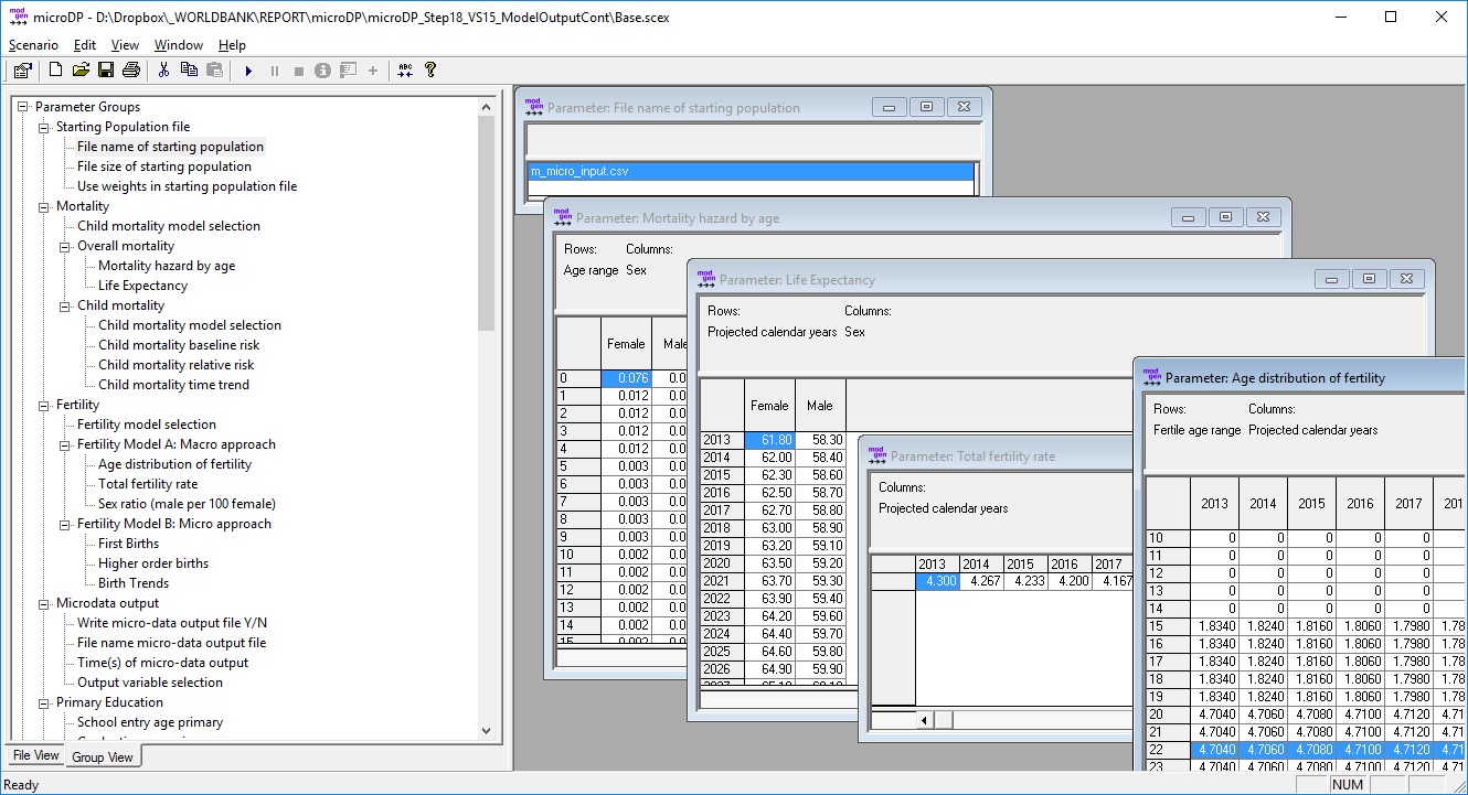
Figure 1-1: The User Interface, Parameter Tables
This screenshot shows the selection of parameter tables essential to the base version of the model: the file name of the starting population, a mortality table, life expectancy, age-specific fertility, and total fertility rate*The user interface is fully documented within the application. The menu offers users access to a detailed hyperlinked help option, which covers relevant aspects, such as editing parameters, creating scenarios, options for running the model, and viewing and exporting model results.
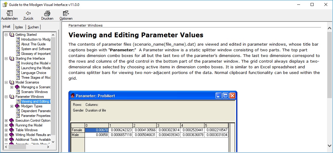
Figure 1-2: The Help Option
Like the user interface, the model is also fully documented within the application. Users can access encyclopedic documentation from the help menu, including descriptions of the modules, parameters, model actors, and all table output.
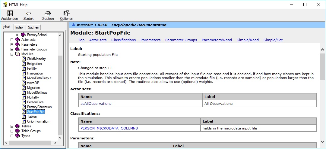
Figure 1-3: The Model Documentation System
- In addition to model parameters, the user also controls some scenario settings. Most importantly, users can choose the time horizon of the simulation and number of replications simulated.
- When running more than one replicate, all model results are automatically calculated as averages over the replicates and distributional information (e.g., the coefficient of variation) is automatically available for each output table cell. This allows users to assess Monte Carlo variation in results.
- The model produces two types of output: a collection of tables and micro-data files for selected moments in time. All tables are updated when running a simulation.
- Tables can have any number of dimensions. For example, population numbers can be displayed by age, year, sex, and province. The user controls how tables are displayed, e.g., a table by age group and year for selected province and sex, or by age group and province for a selected year and sex.
- Like parameter tables, output tables can be opened by clicking on the name in the navigation pane list. For easier navigation, output tables are grouped by topic.
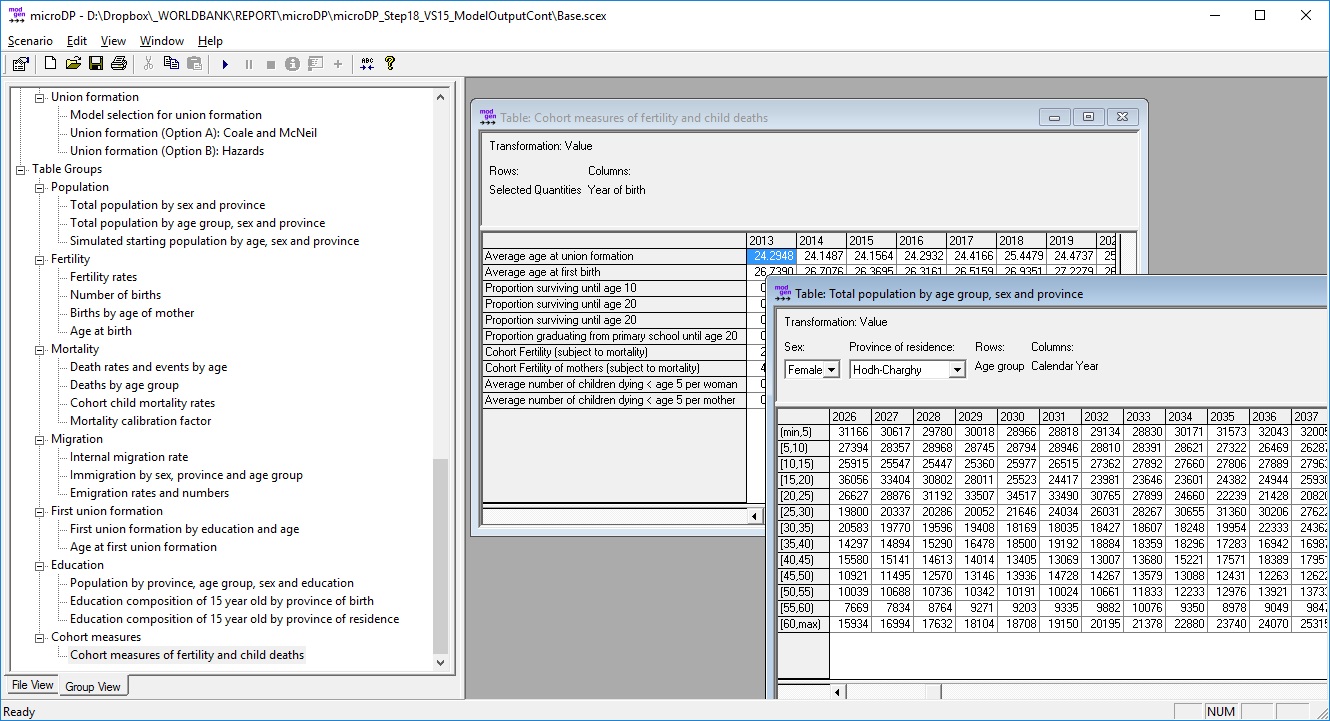
Figure 1-4: Output Tables
1.4.10. Model Output
The model produces a series of tables organized in seven groups. The list of tables can be easily extended by user demand.
Population
- Total population by projected year, sex, and province
- Total population by projected year, age group, sex, and province
- Simulated starting population by age, sex, and province
Fertility
- Age-specific fertility rates by projected year
- Number of births by sex and projected year
- Number of births and first births by age group of mother and projected year
- Average age at birth and at first birth by education and projected year
Mortality
- Death rates and number of deaths by sex, age, and projected year
- Death rates and number of deaths by age group and projected year
- Child mortality by birth cohort and single year of age 0 through 4
- Mortality trends by sex (trend factors calculated internally to scale the standard life table to meet the given scenario of future period life expectancy)
Migration
- Internal migration rates by age group and sex
- Number of immigrants by sex, age group, and province of destination by simulated year
- Emigration rates and number of emigrants by age group, sex, and province by projected year
Union
- First union formation by education, age, and simulated year; rates and proportion of women ever in a union
- Average age at first union formation by education and projected year
Education
- Population by province, age group, sex, and education by projected year
- Education composition of 15-year-old by sex, province of birth, and projected year
- Education composition of 15-year-old by sex, province of residence, and projected year
Female life-course experiences: cohort measures on own survival, union formation, education, fertility, and child deaths
- Average age at union formation
- Average age at first birth
- Proportion surviving until age 10
- Proportion surviving until age 20
- Proportion graduating from primary school
- Cohort Fertility (subject to mortality)
- Cohort Fertility of mothers (subject to mortality)
- Average number of children dying < age 5 per woman
- Average number of children dying < age 5 per mother
1.5. Data Requirements
1.5.1. Overview
Micro-simulation is typically associated with high data demands. This view stems from the predominant use of micro-simulation for modeling highly complex systems, e.g., the operations of social insurance systems in the context of social and demographic change. In contrast to such models, which must depict individual life-courses in great detail and include educational choices, employment, earnings, family dynamics, savings, health, and retirement decisions, the data demands for population projection models are very modest and, for most countries, required data are readily available.
Required data for population projections are life tables for modeling mortality, origin-destination matrices for the modeling migration, and age-specific fertility rates. Here, micro-simulation does not differ from cohort-component models that currently dominate population projections, but the power of micro-simulation is obvious when adding variables and detail. In our application, these variables are primary education, first union formation, and parity—characteristics that allow for a more detailed modeling of the core demographic events. In addition to age, fertility can now account for education, partnership status, and the number and timing of previous births, resulting in the creation of realistic individual life-courses. Concerning mortality, we add a specialized module for child mortality by mother’s characteristics (age and education), and migration now adds education as explanatory variable. As a consequence, the micro-simulation model uses more of the characteristics contained in typical census data, such as education, and will usually require additional information from surveys.
In a nutshell, the micro-simulation population projection presented in this report consists of 11 components and their related data requirements, which collectively add up to 16 variables. Of these components, five are based on the same data as a typical macro projection model:
- Mortality is based on a life table and projected changes of life expectancy. Parameters for mortality are usually available from published data. If no reliable national life table of mortality risks by single year of age is available, a standard life table for the world region can be used. The life table is used for age differences in mortality and automatically calibrated (i.e., re-scaled) to meet the second parameter of the model, life expectancy. Future life expectancy is scenario based.
- Internal migration is based on origin-destination matrices by age group and sex, which can be tabulated from census data. In an optional model extension, education level is added as another dimension; data are typically available from a population census. For easier parameterization and scenario building, the information is split into two tables: (1) the probability to migrate by age group, sex, and province, and (2) the destination of migrants by province of origin, sex, and age group. In the Mauritanian example, the probabilities to leave are modeled using logistic regression assuming the same age patterns in each province. Depending on sample size, these models can be replaced by cross-tabs when running the analysis on the full census. The transition matrices are produced by cross-tabs. In an optional extension, the same model can be parameterized by education group. The education variable is typically available from census data.
- Immigration requires projected total numbers and age distributions by destination province and sex, which can be based on recent numbers, observed in the census, and by applying a time trend.
- Emigration: The emigration module orients itself on typical macro population projection models requiring a single parameter table, namely emigration rates by age group, sex, and province. In the Mauretanian case, emigration was modeled from census information collected on household members who left the country in the past 12 months; there were no other data sources.
- Fertility is based on age-specific fertility rates and projected trends. Current rates can be tabulated from the census. The future age distribution and total fertility rate are scenario based.
The remaining six components require additional information. In the Mauritanian case, three of these models can be estimated from census data alone:
- First union formation uses a parametric (Coale & McNeil) model fitted from census data. The model is parameterized by the earliest age of union formation, average age, and proportion of females eventually entering a union. The parameters are by year of birth and education. Based on the observed proportion of women who have ever entered a union and the age distribution of those observed union formations, curves are fitted that allow projections into the future.
- At its core, the primary education module is based on census data, i.e., the highest level of schooling attended and the highest diploma obtained. An optional extension accounts for mother’s education. The required proportional factor was estimated from MICS.
- The refined version of internal migration uses education as an additional dimension.
The remaining three components require information from survey data. In the Mauritanian case, all additional information is available in MICS data:
The simulation starts from a micro-database—the starting population—which contains nine variables. In the Mauritanian case, all variables but one are available from the census. The file can be the total population or a sample. The most robust available data should be used for the starting population; typically, this would be a population census, a sample thereof, or its synthetic reproduction. Some variables may have to be input from other sources; in the example of Mauritania, a variable was the time of last birth.
WEIGHT          person weight                    e.g., 8.275
BIRTH           time of birth                    e.g., 1966.532
SEX             sex                              0 Female, 1 Male
POR             province of residence            0 .. 12
EDUC            primary education                0 never entered, 1 dropout, 2 completed
POB             province of birth                0 .. 13, (13 for is abroad)
UNION           time of first union (marriage)   e.g. 1988.234
PARITY          number of children ever born      0, 1, ..
LASTBIR         time of last birth               e.g., 2012.34
This additional variable of time at last birth is also used in the refined version of fertility module. Higher-order births were estimated from MICS data, which contain retrospective birth histories that can be used to estimate past time trends. Except for trends, the same models could be estimated from the starting population data set, so they could be mostly based on census data.
The optional infant and child mortality module requires retrospective birth histories and information of deaths as collected from mothers in the MICS survey. Besides an age baseline of child mortality, the model uses relative risks by mother’s characteristics, namely age and education. Estimating these risk factors requires survey data, like the MICS in the Mauritanian case. If not available, relative risks can be borrowed from comparable countries or based on research literature.
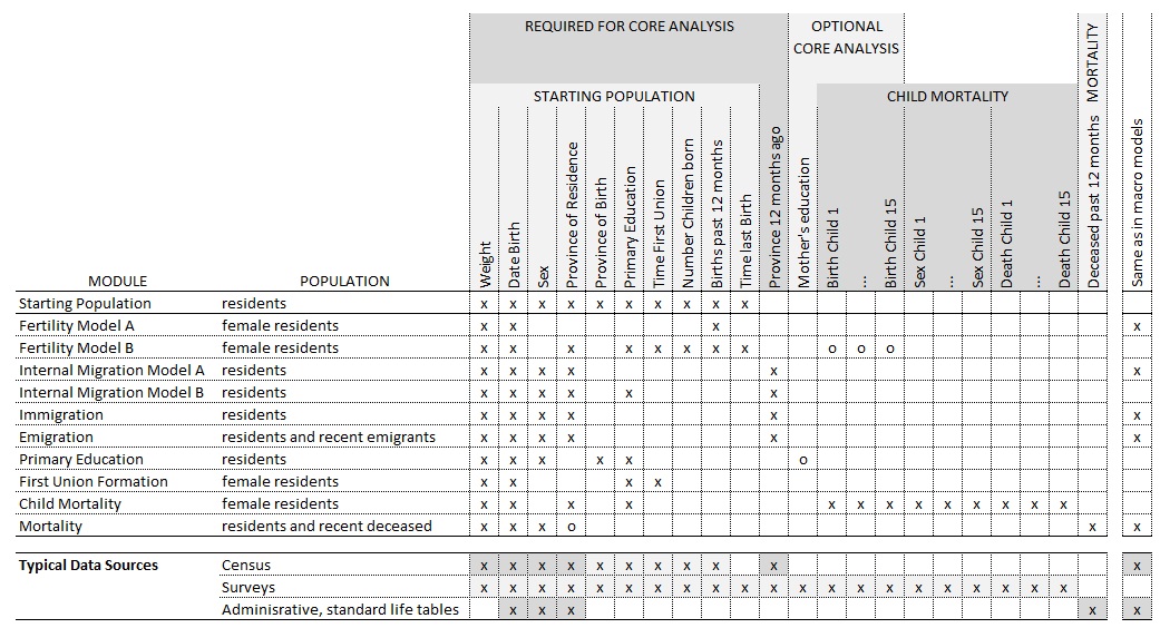
Figure 1-5: Components, Variables, and Data Sources of the Micro-simulation Application (x required; o optional)
1.5.2. Data Files
Population and Housing Census 2013
Most analysis is based on a population census. The following variables and files from the Mauritania 2013 Population and Housing Census (Office Nationale de la Statistique (ONS), Recensement Général de la Population et de l’Habitat (RGPH) 2013) were used for the parametrisation of the model:
CENSUS VARIABLES

- M_WEIGHT                          Weight
- M_AGE                             Age
- M_MALE                            Sex
- M_POB                             Province of birth
- M_POR                             Province of residence
- M_PPROV                           Province 12 months ago
- M_EDUC                            Education (no - enter - finish primary)
- M_AGEMAR                          Age at first marriage
- M_PARITY                          Number of births
- M_BIR12                           Births in past 12 months

CENSUS FILES:

- m_census_residents.dta            A file of residents
- m_census_emigrants.dta            A file of recent (past 12 months) emigrants
- m_census_all_incl_emigrants.dta   The complete file including recent emigrants
- m_census_immigrants               A file of recent (past 12 months) immigrants
The file of recent immigrants was generated from the file of residents and used to adjust immigration to better reflect the number and composition of expected future immigrants. In particular, a large number of recent immigrants were refugees from Mali, an immigration flow that will not continue in the future, according to local experts. Some recent immigrants from Mali were therefore removed from the file.
Emigration was modeled from a file of recent emigrants provided from the National Statistical Office. This file was created from census information on household members who left the country and ignores emigrants who did not leave household members in the country. Other information might be more appropriate and available when porting the model to other countries.
All census analysis files were generated from two samples of raw census data, one on the resident population, the other on recent emigrants.
Multiple Indicator Cluster Survey (MICS) 2011
The Mauritania MICS 2011 (Office Nationale de la Statistique (ONS), Enquête par Grappes à Indicateurs Multiples 2011) was also used for analysis. For higher-order births, an analysis file with the following variables was available or created:
File: m_mics_fertility.dta

Variables:

    - M_ID      Person ID (women)
    - M_BIRTH       Birth date (women)
    - M_WEIGHT      Record Weight
    - M_Bnn     Birth dates of children nn 01-14
    - M_EDUC        Primary education: never entered / dropout / finish level 5+
    - M_MAR     Date of first marriage
Stata file: 11_MICS_CreateAnalysisFile.do
For child mortality, an analysis file with the following variables was available / created:
File: m_mics_childmortality.dta

Variables:

    - M_BIRTH       Date of birth (months since 1900)
    - M_DEATH       Date of death (months since 1900)
    - M_MALE        Sex (Male = 1 / Female = 0)
    - M_WEIGHT      Weight
    - M_AGEMO       Age of mother at birth (in months)
    - M_EDUCMO      Primary education of mother (0 never entered, 1 dropout, 2 graduate)
    - M_INTERV      Date of interview (months since 1900)
Stata code: 15_MICS_CreateAnalysisChildMortality.do